Chapter 13 Basic Mapping
13.1 Outline of Today’s Workshop
We’ll be doing the following few things:
finishing up Spatial Data Handling
discussing finding open-source geospatial data,
then working from this Basic Mapping lab tutorial.
13.2 Spatial Data Handling, fin
There’s a long section in the tutorial about PDF scraping. If you’ve already done it, sorry! I just put together a data package that you can install to use with these tutorials.
Install the package with:
# install.packages("remotes")
remotes::install_github("spatialanalysis/geodaData")
Then, you can pull up the community area data with population attached with:
library(geodaData)
library(sf)
data("chicago_comm")
13.3 Finding Spatial Data
Based on a question from last week, I put together a list with some sources of spatial data.
Question
Question
I’m moving to mapping to make sure we cover the necessary spatial concepts, as some of the exploratory data analysis you may have already encountered. We may go back to the multivariate analysis next week, if time.
Question
13.4 Basic Mapping
We’ll start where we left off last week on Basic Mapping. (We’re running a bit behind schedule, but thank you for asking good questions!)
To use the NYC boundary data included in the tutorial, run the following code:
library(geodaData)
library(sf)
head(nyc_sf)
## Simple feature collection with 6 features and 34 fields
## geometry type: MULTIPOLYGON
## dimension: XY
## bbox: xmin: 913037.2 ymin: 120117 xmax: 1025633 ymax: 230204.7
## epsg (SRID): 2263
## proj4string: +proj=lcc +lat_1=41.03333333333333 +lat_2=40.66666666666666 +lat_0=40.16666666666666 +lon_0=-74 +x_0=300000.0000000001 +y_0=0 +ellps=GRS80 +towgs84=0,0,0,0,0,0,0 +units=us-ft +no_defs
## bor_subb name code subborough forhis06 forhis07
## 1 501 North Shore 501 North Shore 37.0657 34.0317
## 2 502 Mid-Island 502 Mid-Island 27.9822 18.1193
## 3 503 South Shore 503 South Shore 10.7019 12.1404
## 4 401 Astoria 401 Astoria 52.0961 53.9585
## 5 402 Sunnyside / Woodside 402 Sunnyside/Woodside 62.7242 69.3969
## 6 403 Jackson Heights 403 Jackson Heights 68.4834 68.5405
## forhis08 forhis09 forwh06 forwh07 forwh08 forwh09 hhsiz1990 hhsiz00
## 1 27.3767 29.3091 13.2540 11.8768 11.1788 11.1459 2.7146 2.7338
## 2 24.0452 31.1566 20.0616 19.8575 22.4870 17.0371 2.8233 2.7176
## 3 9.6890 14.6638 10.3060 12.7699 9.3561 10.2830 3.0547 2.8497
## 4 54.6968 47.8050 38.3658 35.6551 32.1289 34.6578 2.4279 2.4995
## 5 67.0897 58.2963 37.0512 31.9057 32.3264 33.8794 2.4646 2.6287
## 6 66.5080 69.1580 34.3999 38.2428 38.1470 26.5347 2.8081 3.1650
## hhsiz02 hhsiz05 hhsiz08 kids2000 kids2005 kids2006 kids2007 kids2008
## 1 2.7412 2.8010 2.6983 39.2995 43.3788 38.4022 41.5213 39.8390
## 2 2.5405 2.6228 2.5749 36.2234 35.7630 36.9081 37.6798 37.2447
## 3 2.6525 2.6121 2.6483 39.7362 42.5232 40.3577 40.3797 40.4820
## 4 2.3032 2.3227 2.2746 28.4592 27.2223 25.2556 24.8911 22.0364
## 5 2.5300 2.4993 2.4766 29.8808 28.6841 28.1440 26.3675 29.9032
## 6 2.9108 2.8599 2.8604 41.6335 40.2431 39.3135 37.4414 39.4144
## kids2009 rent2002 rent2005 rent2008 rentpct02 rentpct05 rentpct08
## 1 40.3169 800 900 1000 21.1119 24.8073 28.5344
## 2 37.8176 650 800 950 32.3615 27.2584 27.9567
## 3 35.3880 750 775 800 23.0547 20.4146 18.1590
## 4 17.9996 1000 1100 1400 25.6022 26.7685 28.0467
## 5 26.2156 1000 1000 1400 18.8079 22.6752 21.3009
## 6 39.0377 910 1000 1100 34.0156 34.8050 27.1032
## pubast90 pubast00 yrhom02 yrhom05 yrhom08
## 1 47.32913 6.005791 10.80507 12.12785 11.54743
## 2 35.18232 2.287034 15.24125 15.18311 14.68212
## 3 23.89404 1.350208 12.70425 12.97228 13.56149
## 4 80.53393 5.204510 12.83917 13.37751 12.54464
## 5 75.51687 2.974139 15.38766 12.51879 12.66691
## 6 66.64228 5.332569 12.64923 12.58035 11.96598
## geometry
## 1 MULTIPOLYGON (((962498.9 17...
## 2 MULTIPOLYGON (((928296.9 16...
## 3 MULTIPOLYGON (((932416.3 14...
## 4 MULTIPOLYGON (((1010873 226...
## 5 MULTIPOLYGON (((1011647 216...
## 6 MULTIPOLYGON (((1014790 220...Question
Take a few minutes and try to understand what the NYC data is about.
- How many observations and variables are there? What data is stored? (
dim(),str(),head(),summary()) - What does the metadata tell you about this data? (
?nyc_sf) - What geometries are in this data? Can you make a quick map with
plot()? - What coordinate reference system is there? Is this data projected? (
st_crs()) Can you Google the EPSG code and figure out what it means?
We’ll be working with the tmap R package today. Some resources I find useful for tmap include:
- the tmap examples
- the Geocomputation with R site
Load the library:
library(tmap)tm_shape(nyc_sf) +
tm_polygons("rent2008")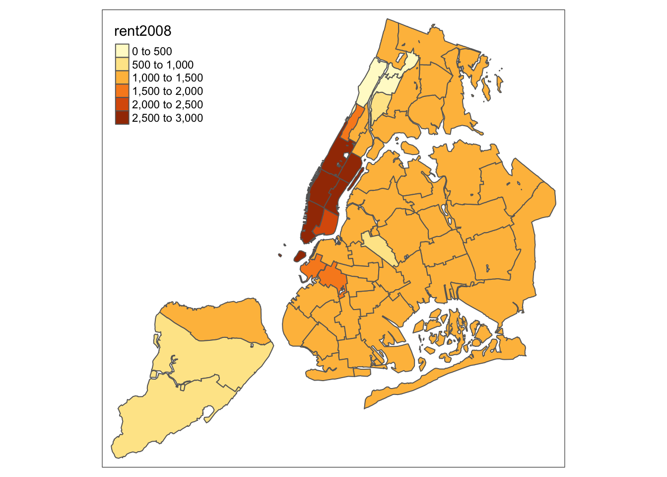
Question
tm_fill() or tm_borders() in place of tm_polygons(). Can you produce the same thing as tm_polygons() with these two functions?
There are multiple ways to do the same thing in R!
In this case, tm_polygons() is a superset of tm_fill() and tm_borders().
13.4.1 Adding a basemap
If you want a basemap for your map, change the tmap_mode to “view”.
tmap_mode("view")## tmap mode set to interactive viewingtm_shape(nyc_sf) +
tm_polygons("rent2008")Want a prettier basemap? R can connect to other map servers. You can preview basemaps and find their names at this Leaflet Provider Demo. You can also pull up a list of all the providers with leaflet::providers.
tm_shape(nyc_sf) +
tm_polygons("rent2008") +
tm_basemap(server = "OpenStreetMap")13.4.2 Customizing tmap function parameters
Each tm_ function has arguments you can set to other things. This allows you to change the color, the transparency, the outlines, the labels, and more. All this customization is very powerful!
Question
tm_polygons with ?tm_polygons? Which parameter controls transparency? How would you change the title of the legend to something else?
I can’t teach you everything in a workshop, so the best thing I can leave you with is an ability to poke through R documentation to find what you need.
13.4.3 Adding a histogram
Certain functionalities are only available in plotting mode, like adding a histogram of the data:
tmap_mode("plot")## tmap mode set to plottingtm_shape(nyc_sf) +
tm_polygons("rent2008", legend.hist = TRUE)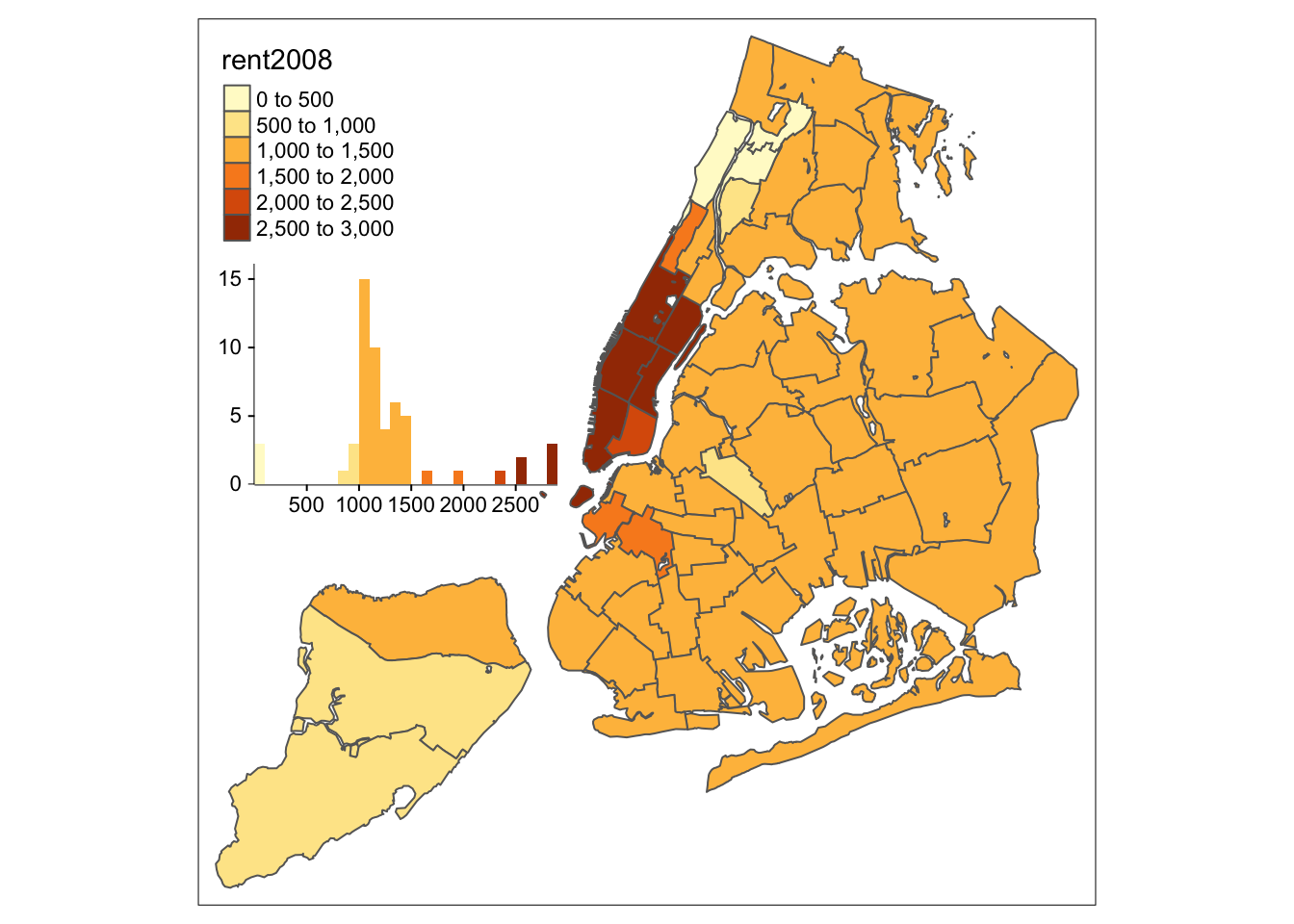
13.4.4 Getting our map ready for production
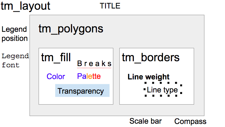
In order to do our final tweaking, we need to do things to the map as a whole. In this case, we’ll use tm_layout(), as we’re not working on one specific aspect of the map.
Question
tm_layout() in the R documentation. (Get ready to be overwhelmed by the options.) What other customizations exist?
We can add a title with title =.
tm_shape(nyc_sf) +
tm_polygons("rent2008", legend.hist = TRUE) +
tm_layout(title = "Rent 2008 NYC Sub-Boroughs")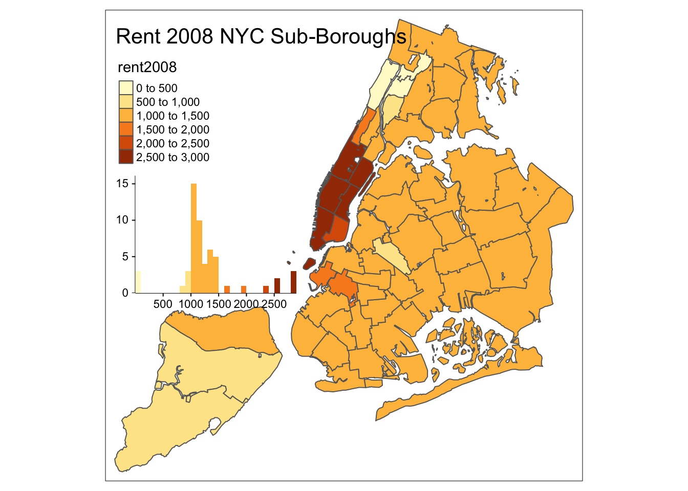
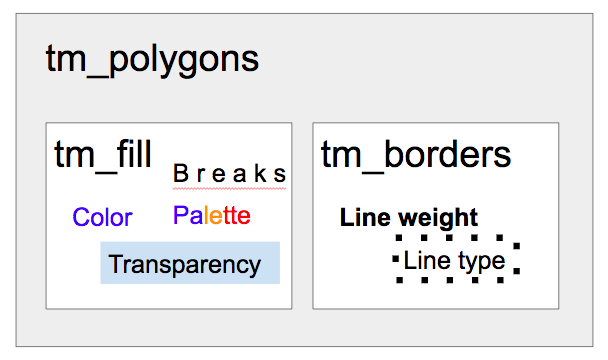
A schematic to clarify how this works:
Question
Try some of the following changes:
- Add a compass and a scale bar
- Move the legend outside
- Move the title outside and center it (try
main.title())
13.4.5 Using Examples
It’s sometimes easier to look for examples, and replicate that code than digging through the documentation.
Question