Chapter 2 Single-Dataset GIS Operations
2.1 Learning Objectives
- Become familiar with several common single-dataset GIS operations
- Calculate centroids of polygons
- Create buffers
- Explore additional single-dataset GIS operations
2.2 Functions Learned
st_geometry()st_centroid()st_buffer()st_coordinates()st_bbox()
2.3 Interactive Tutorial
This workshop’s script can be found here.
2.4 Exercises
- Project 1986 ward data into correct UTM projection
library(sf)
ward86 <- st_read("data/ward1986.shp")
## Reading layer `ward1986' from data source `/Users/angela/Desktop/Spatial Data Science/workshop-notes/data/ward1986.shp' using driver `ESRI Shapefile'
## Simple feature collection with 51 features and 1 field (with 1 geometry empty)
## geometry type: MULTIPOLYGON
## dimension: XY
## bbox: xmin: -87.9402 ymin: 41.6443 xmax: -87.524 ymax: 42.0231
## epsg (SRID): 4269
## proj4string: +proj=longlat +ellps=GRS80 +towgs84=0,0,0,0,0,0,0 +no_defsward86 <- st_transform(ward86, 32616)
plot(ward86)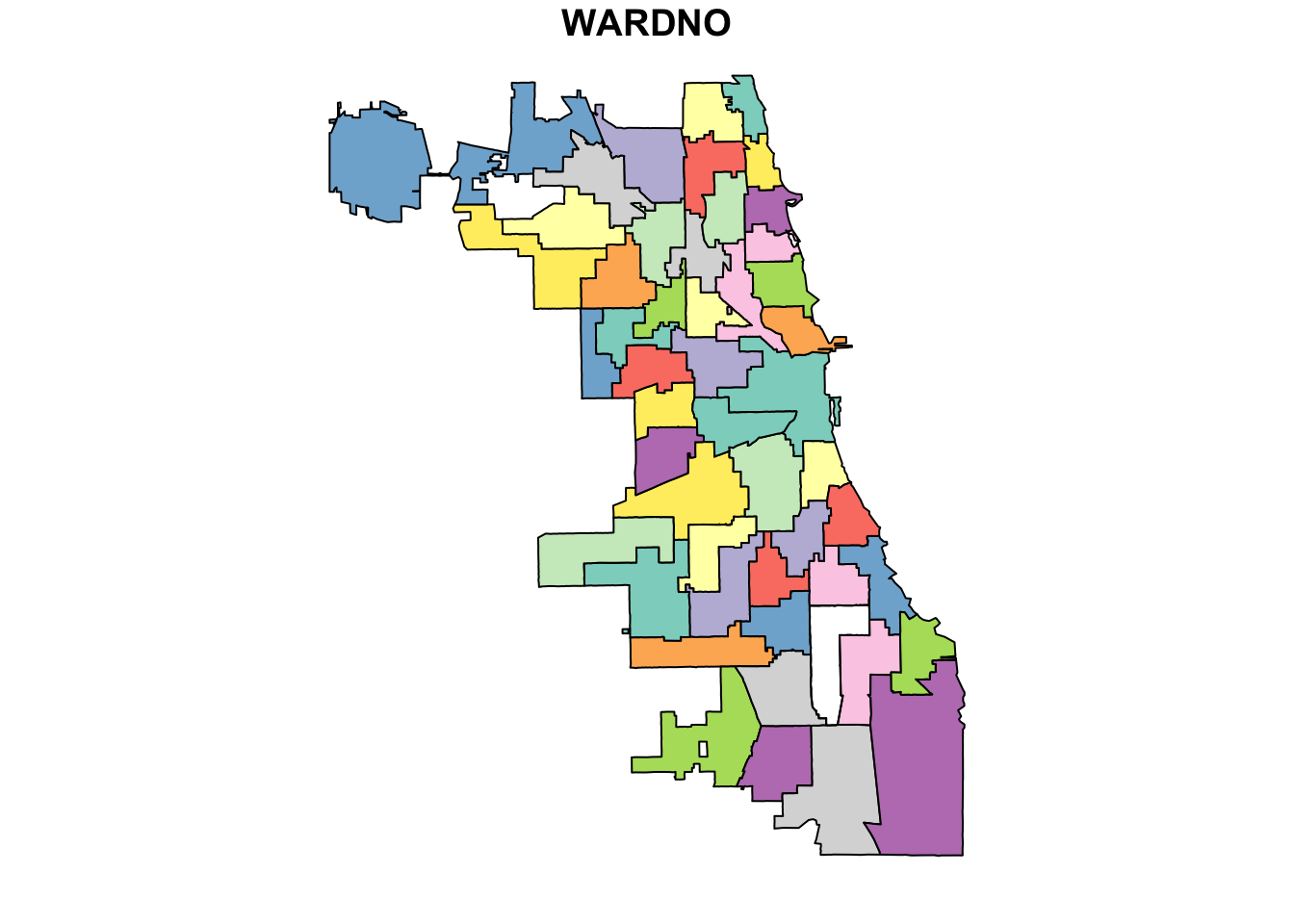
- Calculate centroids of wards with
st_centroid
?st_centroid

centroids <- st_centroid(ward86)
## Warning in st_centroid.sf(ward86): st_centroid assumes attributes are
## constant over geometries of xplot(st_geometry(centroids), cex = 0.1)
plot(st_geometry(ward86), add = T)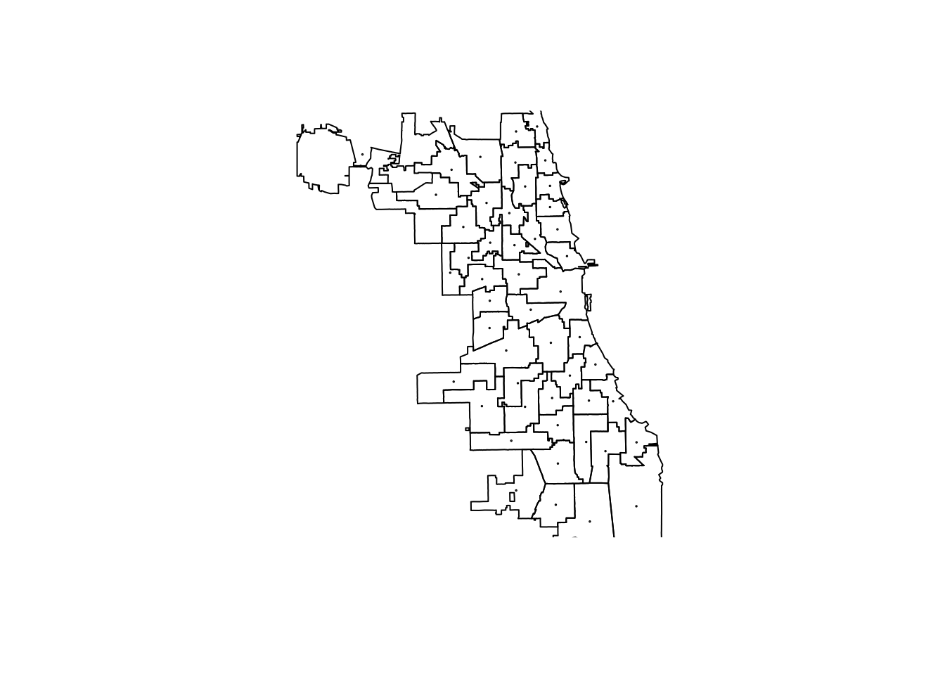
plot(st_geometry(ward86))
plot(st_geometry(centroids), cex = 0.1, add = T)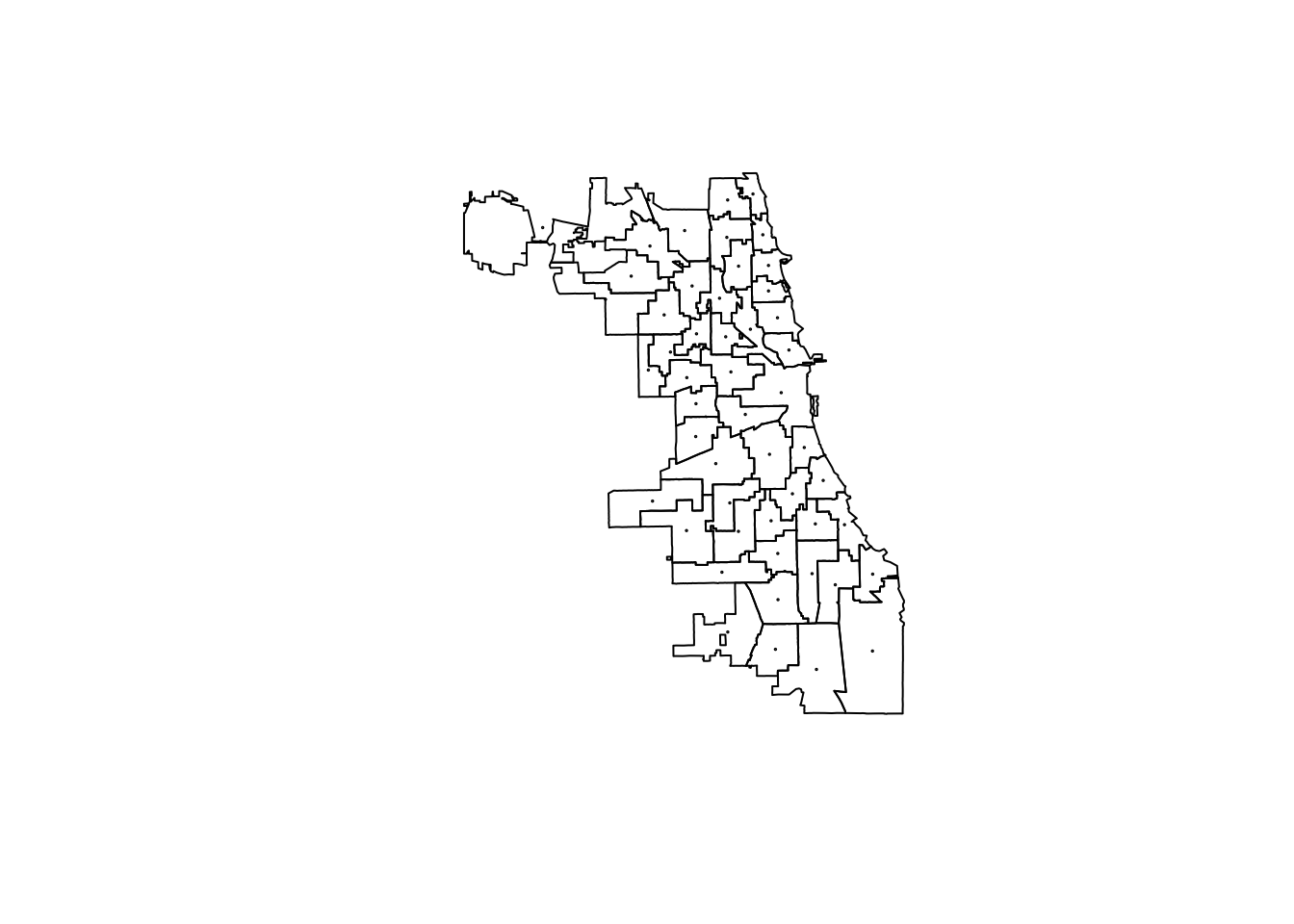
- Calculate bounding box with
st_bbox - Plot centroids, buffered centroids, and wards for each year
2.5 Links
- Geometric unary operations (aka, single dataset operations): https://r-spatial.github.io/sf/reference/geos_unary.html
- sf cheatsheet: https://github.com/rstudio/cheatsheets/blob/master/sf.pdf
- PostGIS cheatsheet (off of which sf is based): http://www.postgis.us/downloads/postgis21_cheatsheet.pdf