Chapter 12 Local Spatial Autocorrelation 1
Introduction
This notebook cover the functionality of the Local Spatial Autocorrelation section of the GeoDa workbook. We refer to that document for details on the methodology, references, etc. The goal of these notes is to approximate as closely as possible the operations carried out using GeoDa by means of a range of R packages.
The notes are written with R beginners in mind, more seasoned R users can probably skip most of the comments on data structures and other R particulars. Also, as always in R, there are typically several ways to achieve a specific objective, so what is shown here is just one way that works, but there often are others (that may even be more elegant, work faster, or scale better).
For this notebook, we use Cleveland house price data. Our goal in this lab is show how to assign spatial weights based on different distance functions.
12.0.1 Objectives
After completing the notebook, you should know how to carry out the following tasks:
Identify clusters with the Local Moran cluster map and significance map
Identify clusters with the Local Geary cluster map and significance map
Identify clusters with the Getis-Ord Gi and Gi* statistics
Identify clusters with the Local Join Count statistic
Interpret the spatial footprint of spatial clusters
Assess potential interaction effects by means of conditional cluster maps
Assess the significance by means of a randomization approach
Assess the sensitivity of different significance cut-off values
Interpret significance by means of Bonferroni bounds
12.0.1.1 R Packages used
spatmap: To construct significance and cluster maps for a variety of local statistics
geodaData: To load the data for this notebook
tmap: To format the maps made
rgeoda: To run local spatial autocorrelation analysis
12.0.1.2 R Commands used
Below follows a list of the commands used in this notebook. For further details and a comprehensive list of options, please consult the R documentation.
Base R:
install.packages,library,setwd,set.seed,cut,reptmap:
tm_shape,tm_borders,tm_fill,tm_layout,tm_facets
12.1 Preliminaries
Before starting, make sure to have the latest version of R and of packages that are compiled for the matching version of R (this document was created using R 3.5.1 of 2018-07-02). Also, optionally, set a working directory, even though we will not actually be saving any files.31
12.1.1 Load packages
First, we load all the required packages using the library command. If you don’t have some of these in your system, make sure to install them first as well as
their dependencies.32 You will get an error message if something is missing. If needed, just install the missing piece and everything will work after that.
library(sf)
library(tmap)
library(rgeoda)
library(geodaData)
library(RColorBrewer)
12.1.2 spatmap
The main package used throughout this notebook will be rgeoda. This package provides the statistical computations of local spatial statistics and tmap for the mapping component. All of the visualizations are built with a similar style
to GeoDa. The visualizations include cluster maps and their associated significance maps. The mapping functions
are built off of tmap and can have additional layers added to them like tm_borders or tm_layout.
12.1.3 geodaData
All of the data for the R notebooks is available in the geodaData
package. We loaded the library earlier, now to access the individual
data sets, we use the double colon notation. This works similar to
to accessing a variable with $, in that a drop down menu will
appear with a list of the datasets included in the package. For this
notebook, we use guerry.
guerry <- geodaData::guerry12.1.4 Univariate analysis
Throughout the notebook, we will focus on the variable Donatns, which is charitable donations per capita. Before proceeding with the local spatial statistics and visualizations, we will take preliminary look at the spatial distribution of this variable. This is done with tmap functions. We will not go into too much detail on these because there is a lot to cover local spatial statistics and this functionality was covered in a previous notebook. Please the Basic Mapping notebook for more information on basic tmap functionality
For the univariate map, we use the natural breaks or jenks style to get a general sense of the spatial distribution for our variable.
tm_shape(guerry) +
  tm_fill("Donatns", style = "jenks", n = 6) +
  tm_borders() +
  tm_layout(legend.outside = TRUE, legend.outside.position = "left")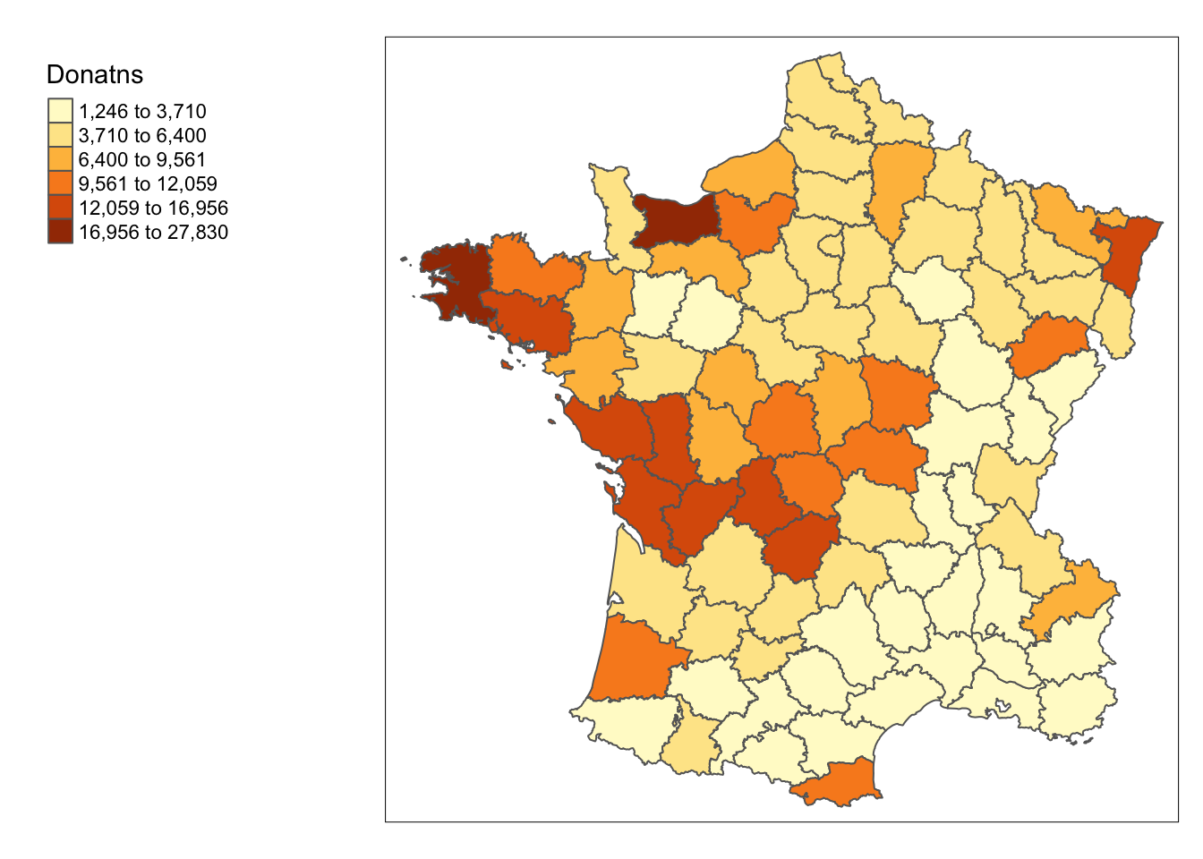
12.2 Local Moran
12.2.1 Principle
The local Moran statistic was suggested in Anselin(1995) as a way to identify local clusters and local spaital outliers. Most global spatial autocorrelation can be expressed as a double sum over i and j indices, such as \(\Sigma_i\Sigma_jg_{ij}\). The local form of such a statistic would then be, for each observation(location)i, the sum of the relevant expression over the j index, \(\Sigma_jg_{ij}\).
Specifically, the local Moran statistic takes the form \(cz_i\Sigma_jw_{ij}z_j\), with z in deviations from the mean. The scalar c is the same for all locations and therefore does not play a role in the assessment of significance. The latter is obtained by means of a conditional permutation method, where, in turn, each \(z_i\) is held fixed, and the remaining z-values are randomly permuted to yield a reference distribution for the statistic. This operates in the same fashion as for the global Moran’s I, except that the permutation is carried out for each observation in turn. The result is a pseudo p-value for each location, which can then be used to assess significance. Note that this notion of significance is not the standard one, and should not be interpreted that way (see the discussion of multiple comparisons below).
Assessing significance in and of itself is not that useful for the Local Moran. However, when an indication of significance is combined with the location of each observation in the Moran Scatterplot, a very powerful interpretation becomes possible. The combined information allows for a classification of the significant locations as high-high and low-low spatial clusters, and high-low and low-high spatial outliers. It is important to keep in mind that the reference to high and low is relative to the mean of the variable, and should not be interpreted in an absolute sense.
12.2.2 Implementation
With the function local_moran from rgeoda, we can create a local moran cluster map. The parameters
needed are an sf dataframe, which is guerry in our case, and the name of a variable from the sf
dataframe.
Some help functions that create maps based the statistical results of rgeoda:
match_palette <- function(patterns, classifications, colors){
  classes_present <- base::unique(patterns)
  mat <- matrix(c(classifications,colors), ncol = 2)
  logi <- classifications %in% classes_present
  pre_col <- matrix(mat[logi], ncol = 2)
  pal <- pre_col[,2]
  return(pal)
}

lisa_map <- function(df, lisa, alpha = .05) {
  clusters <- lisa_clusters(lisa,cutoff = alpha)
  labels <- lisa_labels(lisa)
  pvalue <- lisa_pvalues(lisa)
  colors <- lisa_colors(lisa)
  lisa_patterns <- labels[clusters+1]

  pal <- match_palette(lisa_patterns,labels,colors)
  labels <- labels[labels %in% lisa_patterns]

  df["lisa_clusters"] <- clusters
  tm_shape(df) +
    tm_fill("lisa_clusters",labels = labels, palette = pal,style = "cat")
}

significance_map <- function(df, lisa, permutations = 999, alpha = .05) {
  pvalue <- lisa_pvalues(lisa)
  target_p <- 1 / (1 + permutations)
  potential_brks <- c(.00001, .0001, .001, .01)
  brks <- potential_brks[which(potential_brks > target_p & potential_brks < alpha)]
  brks2 <- c(target_p, brks, alpha)
  labels <- c(as.character(brks2), "Not Significant")
  brks3 <- c(0, brks2, 1)

  cuts <- cut(pvalue, breaks = brks3,labels = labels)
  df["sig"] <- cuts

  pal <- rev(brewer.pal(length(labels), "Greens"))
  pal[length(pal)] <- "#D3D3D3"

  tm_shape(df) +
    tm_fill("sig", palette = pal)
}
It is important to note the default parameters of local_moran. These include permutations = 999,
significance_cutoff = .05, and weights = NULL. Permutations is the number of permutations used in computing the reference distributions
of the local statistic for each location. Significance_cutoff or alpha is the cutoff significance level. The weights parameter is where we specify
the weights used for the computation of the local statistics. In the NULL case, 1st order queen contiguity are computed.
w <- queen_weights(guerry)
lisa <- local_moran(w, guerry['Donatns'])
lisa_map(guerry, lisa)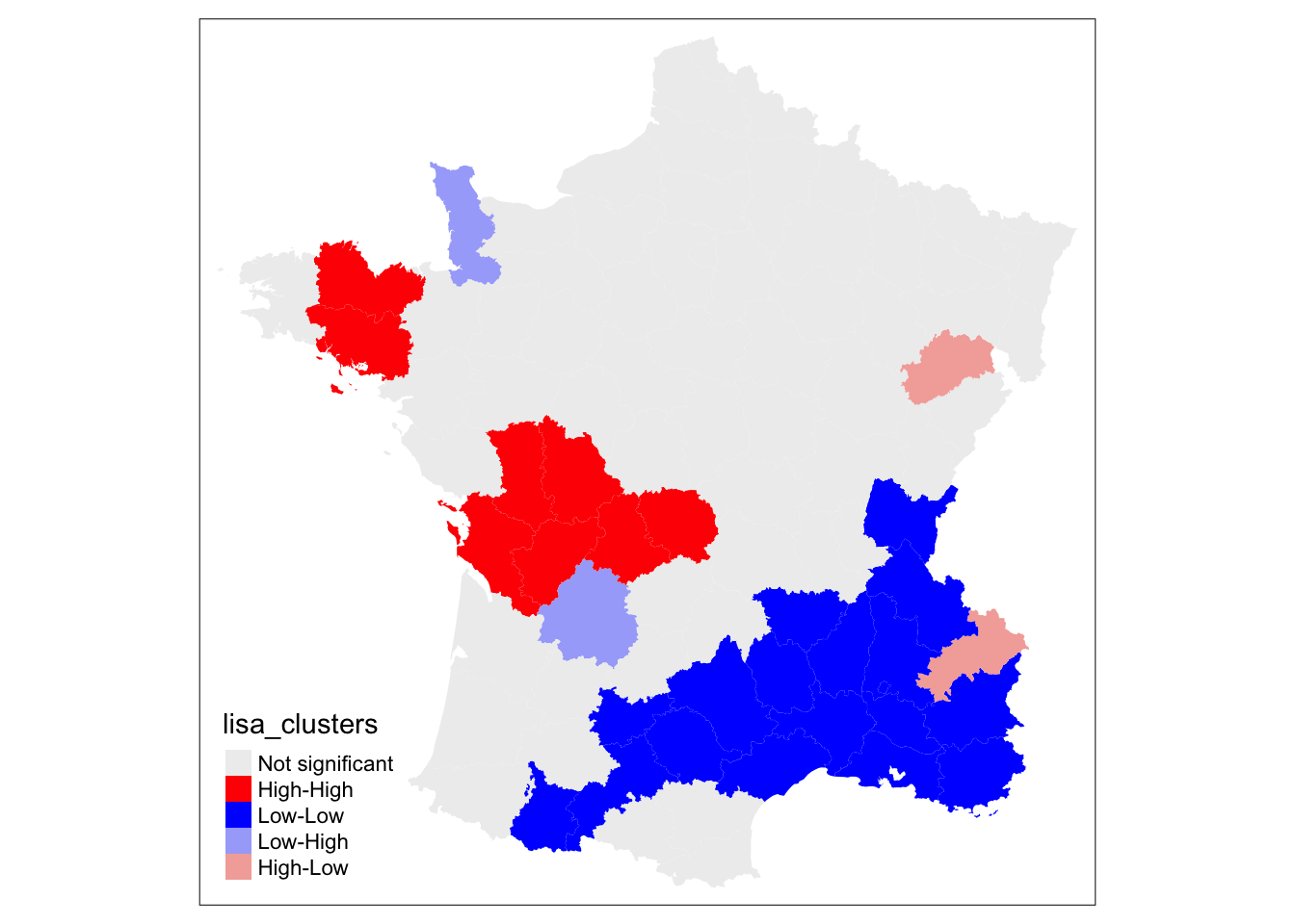
To get a significance map for the local moran, we use significance_map. Default number of permutations is 999,
the alpha level is .05.
significance_map(guerry, lisa) 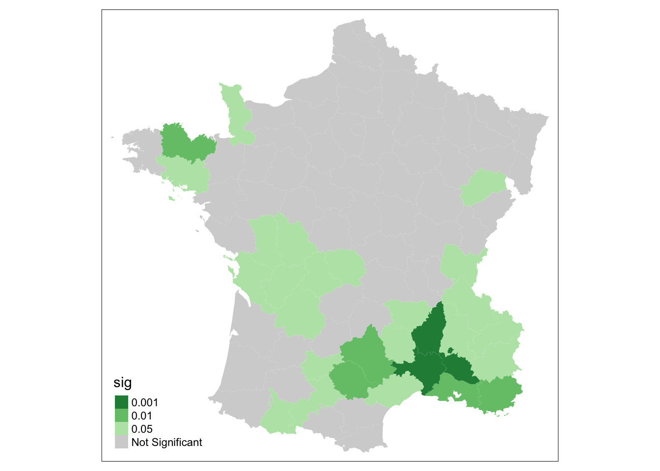
12.2.2.1 tmap additions
With the mapping functions of lisa_map, additional tmap layers can be added
with the + operator. This gives the maps strong formatting options. With tm_borders,
we can make the borders of the local moran map more distinct. Withtm_layout we can add
a title and move the legend to the outside of the map. There many more formatting options,
including tmap_arrange, which we used earlier.
lisa_map(guerry, lisa) +
  tm_borders() +
  tm_layout(title = "Local Moran Cluster Map of Donatns", legend.outside = TRUE)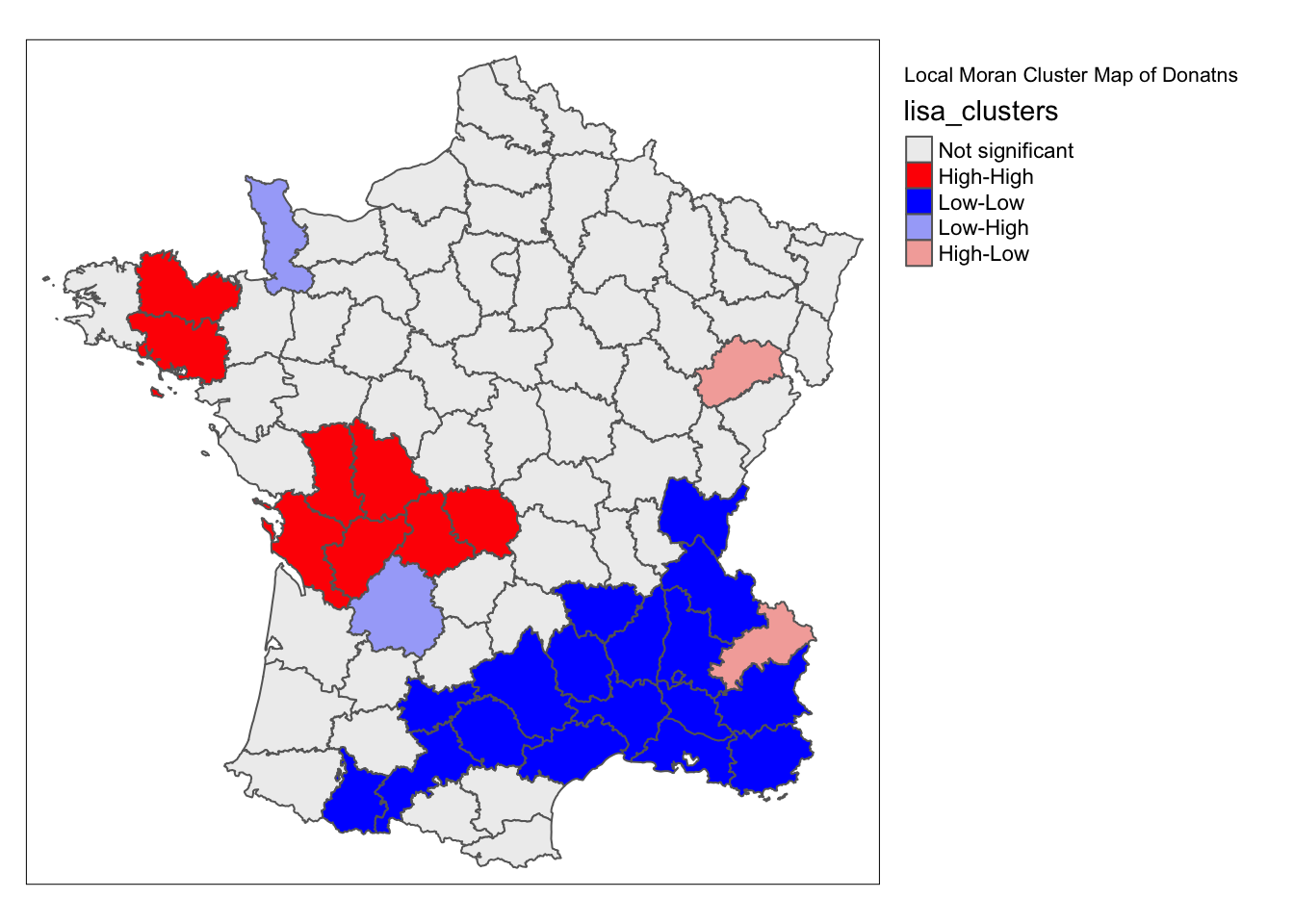
We can set the tmap mode to “view”” to get an interactive base map with tmap_mode.
tmap_mode("view")
lisa_map(guerry, lisa) +
  tm_borders() +
  tm_layout(title = "Local Moran Cluster Map of Donatns",legend.outside = TRUE)
We set tmap_mode("plot") to get normal maps for the rest of the notebook. While basemaps are a nice
option, they are not necessary for the remainder of the notebook.
tmap_mode("plot")12.2.3 Randomization Options
To obtain higher significance levels, we need to use more permutations in the computation
of the the local moran for each location. For instance, a pseudo pvalue of .00001 would
require 999999 permutations. To get more permutations, we set permutations = 99999 in
local_moran. It is important to note that the maximum number of permutations for this function is 99999.
lisa <- local_moran(w, guerry['Donatns'], permutations = 99999)
lisa_map(guerry, lisa) +
  tm_borders() +
  tm_layout(title = "Local Moran Cluster Map of Donatns", legend.outside = TRUE)
For the significance map, the process is the same, we set permutations = 99999.
significance_map(guerry, lisa, permutations = 99999) +
  tm_borders() +
  tm_layout(title = "Local Moran Significance Map of Donatns", legend.outside = TRUE)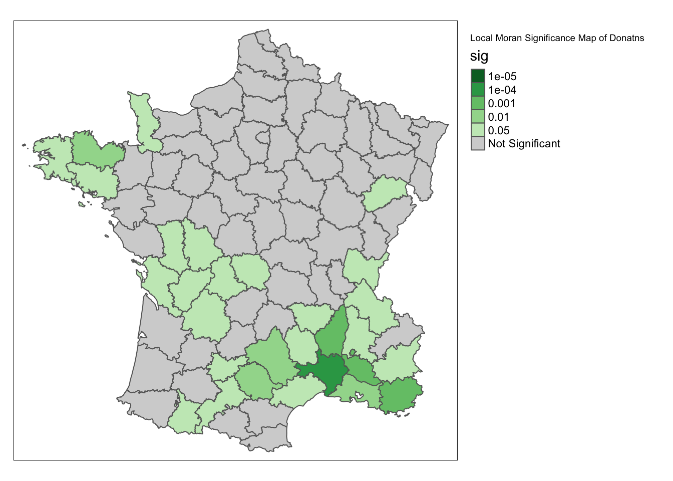
12.2.4 Significance
An important methodological issue associated with the local spatial autocorrelation statistics is the selection of the p-value cut-off to properly reflect the desired Type I error. Not only are the pseudo p-values not analytical, since they are the result of a computational permutation process, but they also suffer from the problem of multiple comparisons. The bottom line is that a traditional choice of 0.05 is likely to lead to many false positives, i.e., rejections of the null when in fact it holds.
To change the cut-off level of significance in the local moran cluster mapping function we use the
parameter alpha =. The default option is .05, but if we want another level, say .01, we set
alpha = .01.
lisa_map(guerry, lisa, alpha = .01) +
  tm_borders() +
  tm_layout(title = "Local Moran Cluster Map of Donatns", legend.outside = TRUE)
The process is the same in significance_map, we set alpha = .01.
significance_map(guerry, lisa, permutations = 99999, alpha = .01) +
  tm_borders() +
  tm_layout(title = "Local Moran Significance Map of Donatns", legend.outside = TRUE)
12.2.4.1 Bonferroni bound
The Bonferroni bound constructs a bound on the overall p-value by taking \(\alpha\) and
dividing it by the number of comparisons. In our context, the latter corresponds to the
number of observation, n. As a result, the Bonferroni bound would be \(\alpha/n = .00012\),
the cutoff p-value to be used to determine significance. We assign bonferroni to be
.01 / 85. Then we use lisa_map with permutations = 99999 and alpha = bonferroni. This
will give us a local moran cluster map with a bonferroni significance cut-off.
bonferroni <- .01 / 85
lisa_map(guerry, lisa, alpha = bonferroni) +
  tm_borders() +
  tm_layout(title = "Local Moran Cluster Map of Donatns", legend.outside = TRUE)
To make the significance map with the bonferroni bound, we set alpha = bonferroni.
significance_map(guerry, lisa,permutations = 99999, alpha = bonferroni) +
  tm_borders() +
  tm_layout(title = "Local Moran Significance Map of Donatns", legend.outside = TRUE)
12.2.4.2 Interpretation of significance
As mentioned, there is no fully satisfactory solution to deal with the multiple comparison problem. Therefore, it is recommended to carry out a sensitivity analysis and to identify the stage where the results become interesting. A mechanical use of 0.05 as a cut off value is definitely not the proper way to proceed.
Also, for the Bonferroni procedure to work properly, it is necessary to have a large number of permutations, to ensure that the minimum p-value can be less than \(\alpha/n\). The maximum number of permutations supported is 99999. The bonferroni approach will be limited for datasets with many locations. With \(\alpha = .01\), datasets with n > 1000, cannot yield significant locations.
12.2.5 Interpretation of clusters
Strictly speaking, the locations shown as significant on the significance and cluster maps are not the actual clusters, but the cores of a cluster. In contrast, in the case of spatial outliers, they are the actual locations of interest.
12.2.6 Conditional local cluster maps
To make the conditional map, we first need to make two categorical variables, with two categories.
cut breaks the data up into two equal pieces. With the two categorical variables, we can create
facets with tmap.
guerry$cut.literacy <- cut(guerry$Litercy, breaks = 2)
guerry$cut.clergy <- cut(guerry$Clergy, breaks = 2)
To make conditional maps, the only addition needed is tm_facets, which will use the two categorical variables created
above. We set by = c("cut.literacy","cut.clergy"). This will give use four maps faceted by the two categorical variables
that we made above.
lisa_map(guerry, lisa) +
  tm_borders() +
  tm_facets(by = c("cut.literacy","cut.clergy"),free.coords = FALSE,drop.units=FALSE)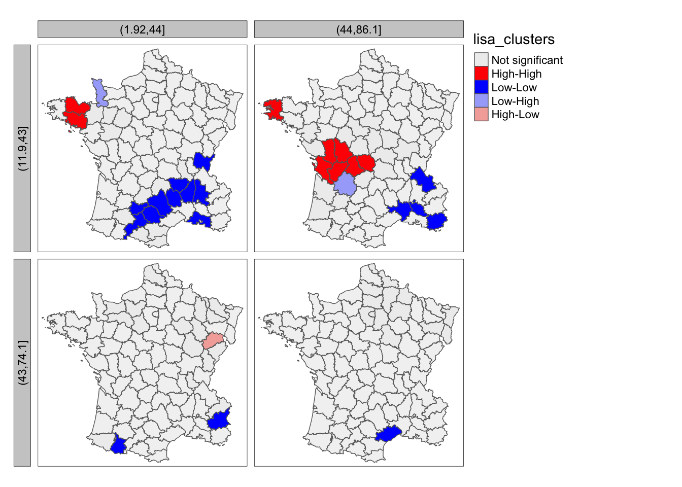
12.3 Local Geary
12.3.1 Principle
The Local Geary statistic, first outlined in Anselin (1995), and further elaborated upon in Anselin (2018), is a Local Indicator of Spatial Association (LISA) that uses a different measure of attribute similarity. As in its global counterpart, the focus is on squared differences, or, rather, dissimilarity. In other words, small values of the statistics suggest positive spatial autocorrelation, whereas large values suggest negative spatial autocorrelation.
Formally, the Local Geary statistic is
\[LG_i = \Sigma_jw_{ij}(x_i-x_j)^2\]
in the usual notation.
Inference is again based on a conditional permutation procedure and is interpreted in the same way as for the Local Moran statistic. However, the interpretation of significant locations in terms of the type of association is not as straightforward. In essence, this is because the attribute similarity is not a cross-product and thus has no direct correspondence with the slope in a scatter plot. Nevertheless, we can use the linking capability within GeoDa to make an incomplete classification.
Those locations identified as significant and with the Local Geary statistic smaller than its mean, suggest positive spatial autocorrelation (small differences imply similarity). For those observations that can be classified in the upper-right or lower-left quadrants of a matching Moran scatter plot, we can identify the association as high-high or low-low. However, given that the squared difference can cross the mean, there may be observations for which such a classification is not possible. We will refer to those as other positive spatial autocorrelation.
For negative spatial autocorrelation (large values imply dissimilarity), it is not possible to assess whether the association is between high-low or low-high outliers, since the squaring of the differences removes the sign.
12.3.2 Implementation
For the local geary map, we use loca_geary(). It has the same default parameters with 999 permutations, an alpha level of .05, and 1st order queen contiguity weights. For mapping function lisa_map(), the inputs are the
same as lisa_map with an sf dataframe: guerry, and the results of local_geary(): lisa. We can
add tmap layers to this mapping function too. Here we use tm_borders and tm_layout
lisa <- local_geary(w, guerry['Donatns'])
lisa_map(guerry, lisa) +
  tm_borders() +
  tm_layout("Local Geary Cluster Map", legend.outside = TRUE)
To get the significance map that directly corresponds with the Local Geary map, the random seed needs to be the same and set before each function, as with the moran.
significance_map(guerry,lisa) +
  tm_borders() +
  tm_layout("Local Geary Significance Map", legend.outside = TRUE)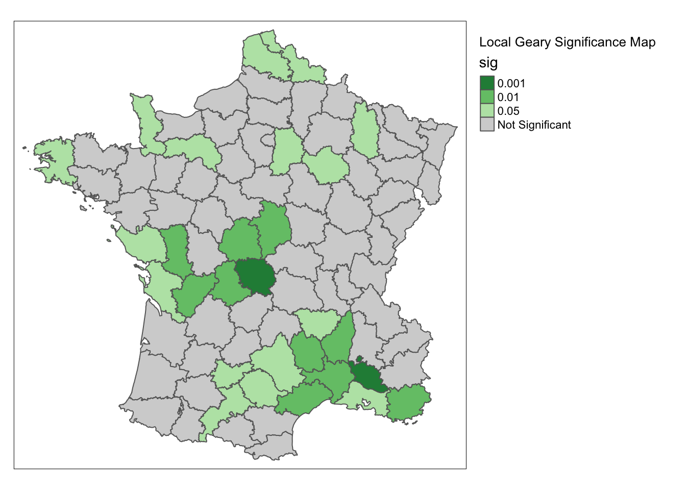
12.3.2.1 Interpretation and significance
To get more permutations, we set permutations = 99999
lisa <- local_geary(w, guerry['Donatns'], permutations = 99999)
lisa_map(guerry, lisa)  +
  tm_borders() +
  tm_layout("Local Geary Cluster Map", legend.outside = TRUE)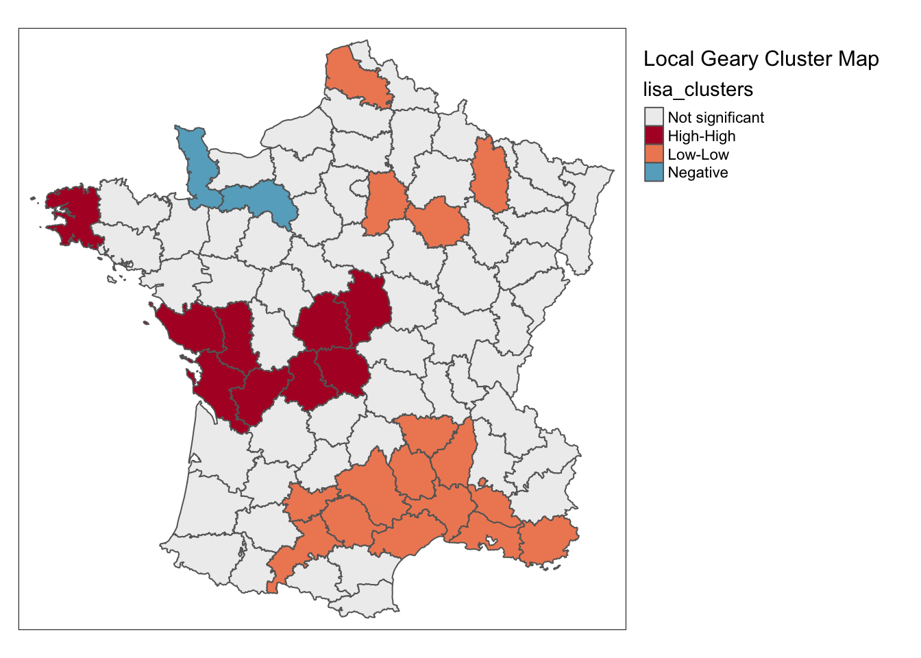
We do the same thing to get more permutations for the significance map.
significance_map(guerry, lisa,permutations = 99999) +
  tm_borders() +
  tm_layout("Local Geary Significance Map", legend.outside = TRUE)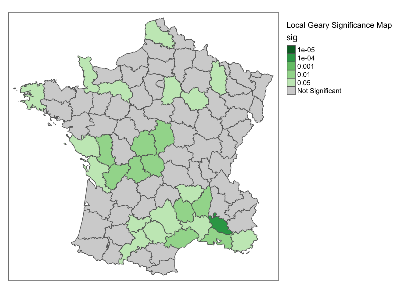

12.4 Getis-Ord Statistics
12.4.1 Principle
A third class of statistics for local spatial autocorrelation was suggested by Getis and Ord (1992), and further elaborated upon in Ord and Getis (1995). It is derived from a point pattern analysis logic. In its earliest formulation the statistic consisted of a ratio of the number of observations within a given range of a point to the total count of points. In a more general form, the statistic is applied to the values at neighboring locations (as defined by the spatial weights). There are two versions of the statistic. They differ in that one takes the value at the given location into account, and the other does not.
The \(G_i\) statistic consists of a ratio of the weighted average of the values in the neighboring locations, to the sum of all values, not including the value at the location \(x_i\)
\[G_i = \frac{\Sigma_{j\neq i}w_{ij}x_j}{\Sigma_{j\neq i}x_j}\]
In contrast, the \(G_i^*\) statistic includes the value \(x_i\) in numerator and denominator:
\[G_i^*=\frac{\Sigma_jw_{ij}x_j}{\Sigma_jx_j}\]
Note that in this case, the denominator is constant across all observations and simply consists of the total sum of all values in the data set.
The interpretation of the Getis-Ord statistics is very straightforward: a value larger than the mean (or, a positive value for a standardized z-value) suggests a high-high cluster or hot spot, a value smaller than the mean (or, negative for a z-value) indicates a low-low cluster or cold spot. In contrast to the Local Moran and Local Geary statistics, the Getis-Ord approach does not consider spatial outliers.
Inference is based on conditional permutation, using an identical procedure as for the other statistics.
12.4.2 Implementation
We can make a cluster map for the local G statistic with loca_g(). The formatting, parameters, and default options
are the same with this function as the other mapping functions in rgeoda.
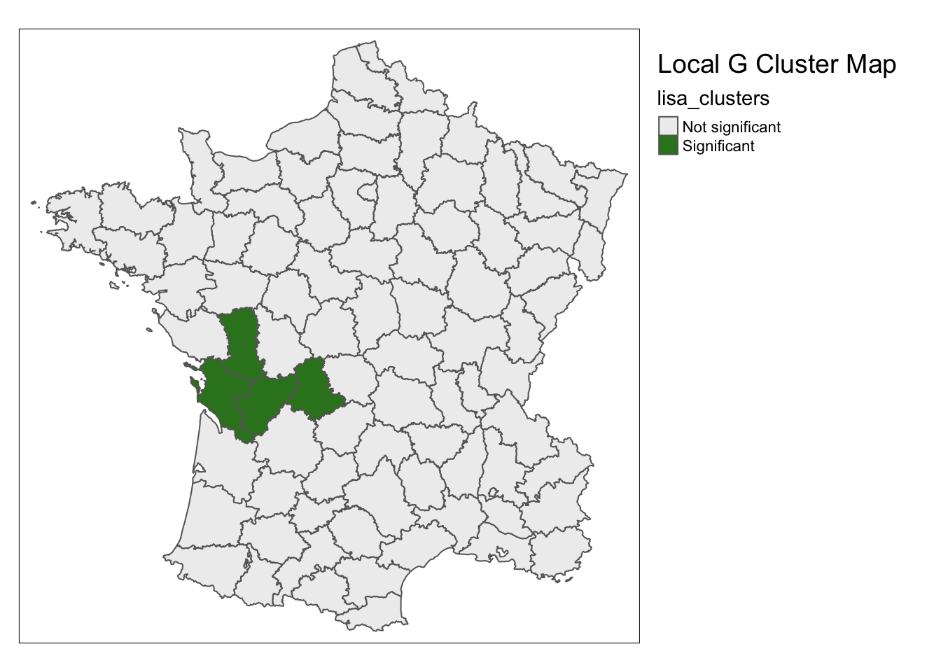
lisa <- local_g(w, guerry['Donatns'])
lisa_map(guerry,  lisa) +
  tm_borders() +
  tm_layout(title = "Local G Cluster Map",legend.outside = TRUE)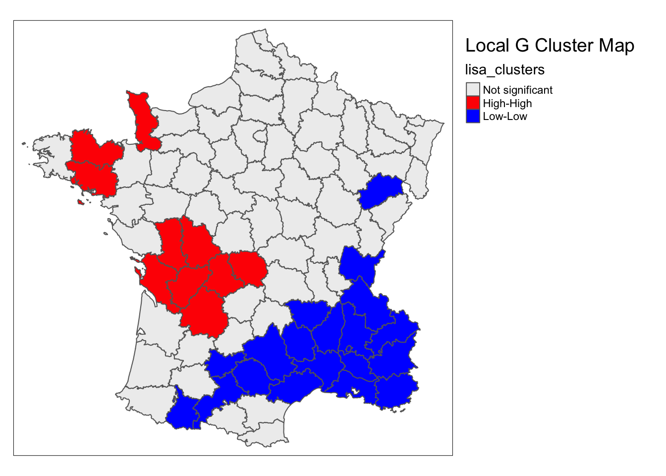
To make the \(G*\) cluster map, we run local_gstar().
lisa <- local_gstar(w, guerry['Donatns'])
lisa_map(guerry, lisa) +
  tm_borders() +
  tm_layout(title = "Local G* Cluster Map",legend.outside = TRUE)
For the significance map, we use significance_map.
significance_map(guerry, lisa) +
  tm_borders() +
  tm_layout(title = "Local G Significance Map",legend.outside = TRUE)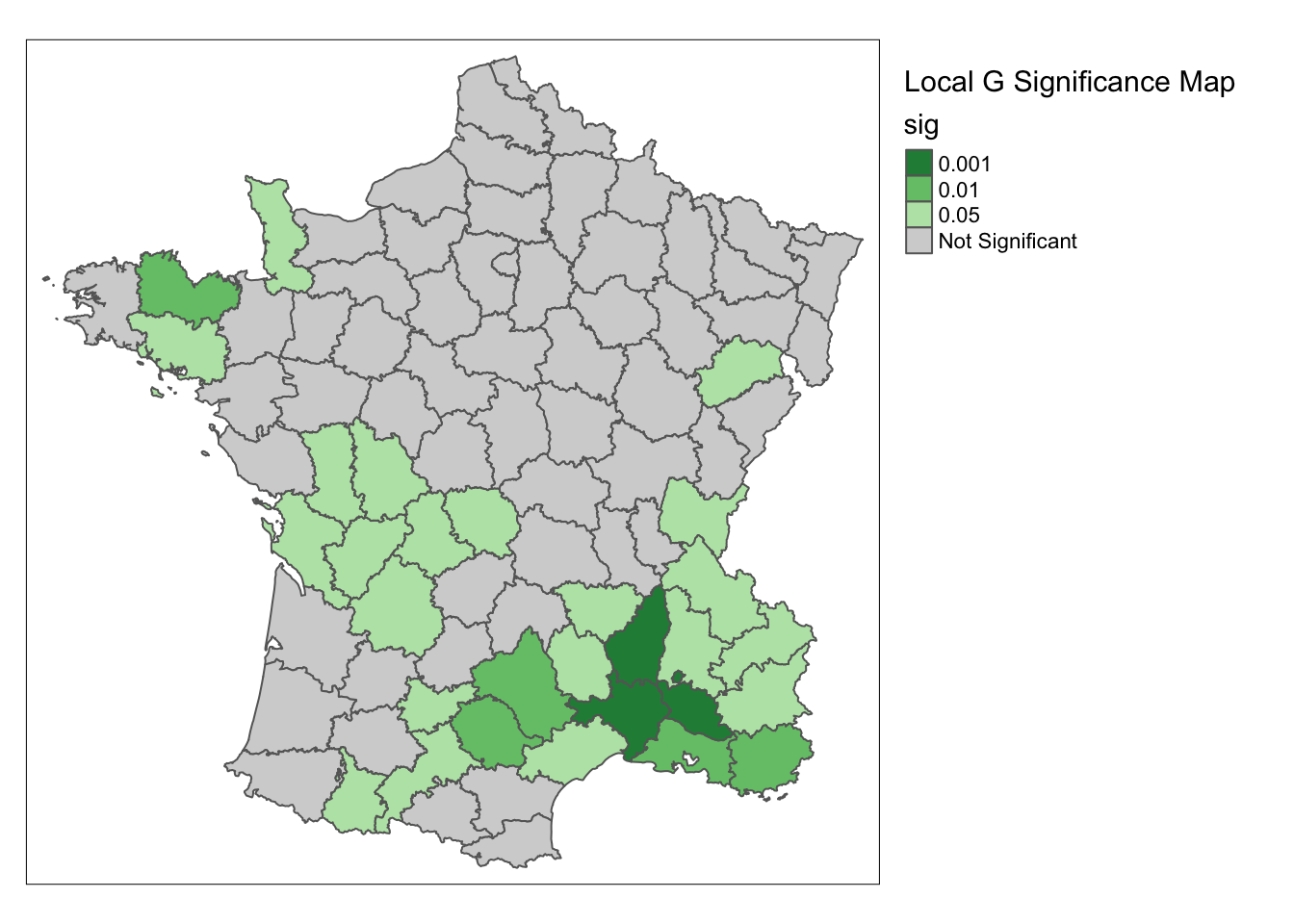
12.4.3 Interpretation and significance
To change the permutations and the cut-off significance level, we use permutation =, and alpha =. The
default options for these parameters are 999 for permutations and .05 for alpha, as with the other
spatmap mapping functions. Here we change permutations = 99999 and alpha = .01.
lisa_map(guerry, lisa, alpha = .01) +
  tm_borders() +
  tm_layout(title = "Local G Cluster Map",legend.outside = TRUE)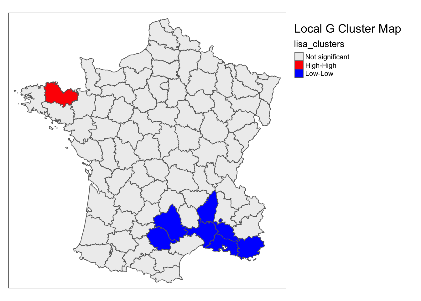
The process is the same for the corresponding significance map. Increasing the permutations gives us more detailed information about the significance at each location.
significance_map(guerry, lisa, permutations = 99999,alpha = .01) +
  tm_borders() +
  tm_layout(title = "Local G Significance Map",legend.outside = TRUE)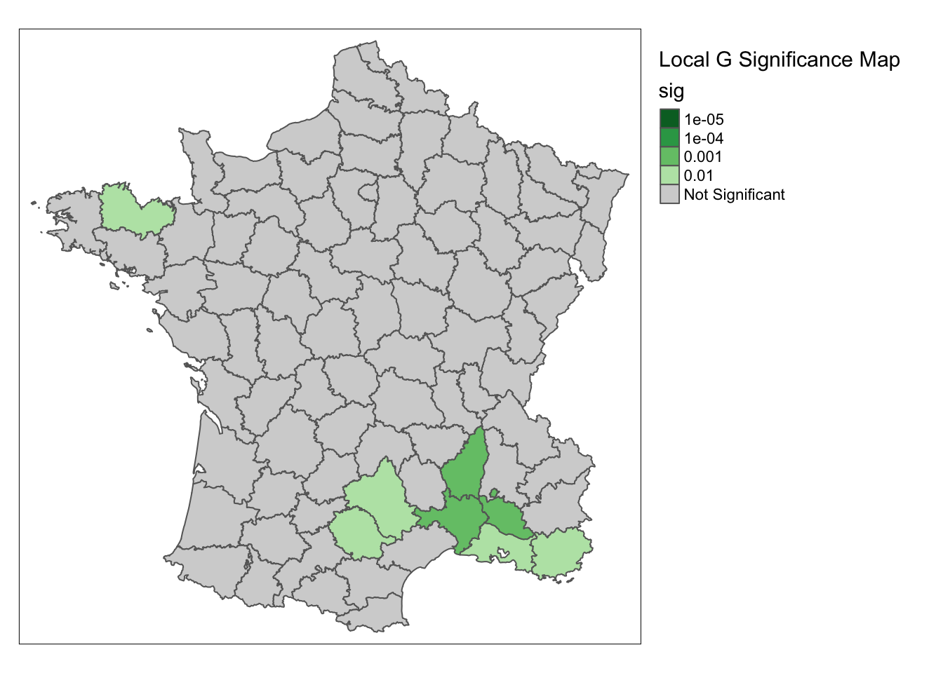
12.5 Local Join Count Statistic
12.5.1 Principle
Recently, Anselin and Li (2019) showed how a constrained version of the \(G_i^*\) statistic yields a local version of the well-known join count statistic for spatial autocorrelation of binary variables, popularized by Cliff and Ord (1973). Expressed as a LISA statistic, a local version of the so-called BB join count statistic is
\[BB_i = x_i\Sigma_jw_{ij}x_j\]
where \(x_{i,j}\) can only take on the values of 1 and 0, and \(w_{ij}\) are the elements of a binary spatial weights matrix (i.e., not row-standardized). For the most meaningful results, the value of 1 should be chosen for the case with the fewest observations (of course, the definition of what is 1 and 0 can easily be switched).
The statistic is only meaningful for those observations where \(x_i =1\), since for \(x_i =0\) the result will always equal zero. A pseudo p-value is obtained by means of a conditional permutation approach, in the same way as for the other local spatial autocorrelation statistics, but only for those observations with \(x_i=1\). The same caveats as before should be kept in mind when interpreting the results, which are subject to multiple comparisons and the sensitivity of the pseudo p-value to the actual simulation experiment (random seed, number of permutations). Technical details are provided in Anselin and Li (2019).
12.5.2 Implementation
Since the local join count only uses binary variables(numeric variables of 1 or 0), we must make one
for guerry. To get the number of observations in guerry we use nrow. We create and empty vector
of 0’s of length n with rep. We assign 1 for the locations that have Donatns greater than 10996.
Lastly we add the binary variable doncat to the sf dataframe.
n <- nrow(guerry)
doncat <- rep(0, n)
doncat[guerry$Donatns > 10996] <- 1
guerry$doncat <- doncat
We map these locations using tmap functions. We set style = "cat" because the variable is and only has two
possible values. We use color white for 0 and color blue for 1.
tm_shape(guerry) +
  tm_fill("doncat", style = "cat", palette = c("white", "blue")) +
  tm_borders() +
  tm_layout(legend.outside = TRUE)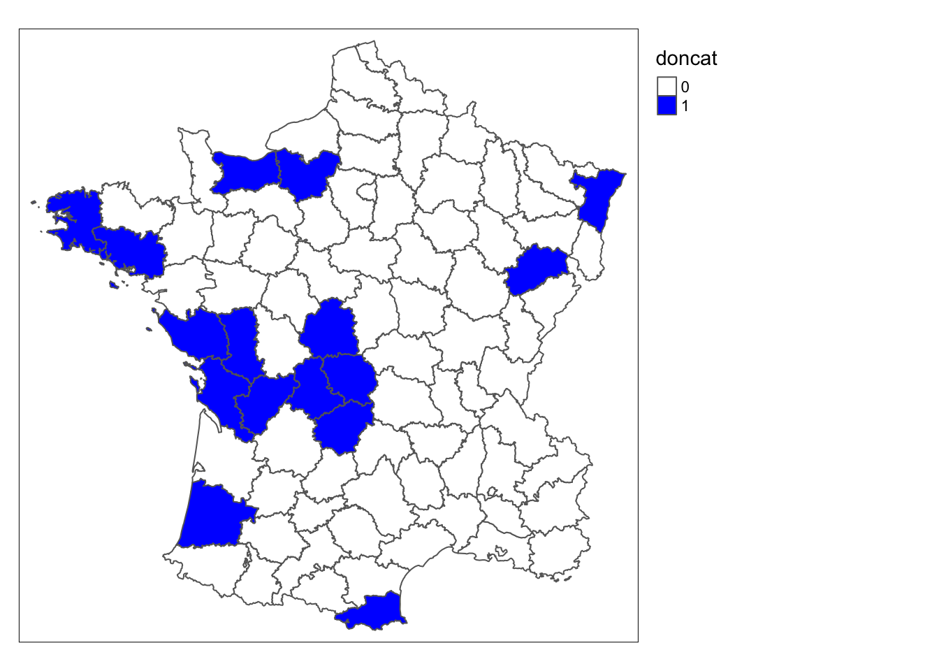
To make the local join count cluster map, we use local_joincount() with doncat as the input variables. We change
permutations to be 99999. This function has the same default options and paramters as the other mapping functions.
lisa <- local_joincount(w, guerry['doncat'], permutations = 99999)
lisa_map(guerry, lisa) +
  tm_borders() +
  tm_layout(title = "Local G Cluster Map",legend.outside = TRUE)