Introduction
This notebook cover the functionality of the Distance-Based Spatial Weights section of the GeoDa workbook. We refer to that document for details on the methodology, references, etc. The goal of these notes is to approximate as closely as possible the operations carried out using GeoDa by means of a range of R packages.
The notes are written with R beginners in mind, more seasoned R users can probably skip most of the comments on data structures and other R particulars. Also, as always in R, there are typically several ways to achieve a specific objective, so what is shown here is just one way that works, but there often are others (that may even be more elegant, work faster, or scale better).
For this notebook, we use Cleveland homesale point data. Our goal in this lab is show how to implement distance-band spatial weights
Objectives
After completing the notebook, you should know how to carry out the following tasks:
Construct distance band spatial weights
Assess the characteristics of distance-based weights
Assess the effect of the max-min distance cut-off
Identify isolates
Construct k-nearest neighbor spatial weights
Create Thiessen polygons from a point layer
Construct contiguity weights for points and distance weights for polygons
Understand the use of great circle distance
R Packages used
tmap: To plot our points on a base map
sf: Used to read the shapefiles in, make contiguity weights, and convert from sp,
spdep: Used to create distance neighbors and contiguity neighbors
ggplot2: To make connectivity histograms
deldir: To make Thiessen polygons.
sp: Used to get an intermediate data structure to get the Thiessen polygons to sf class
_ purr: Used for a mapping function
- geodaData: To get the data for this notebook
R Commands used
Below follows a list of the commands used in this notebook. For further details and a comprehensive list of options, please consult the R documentation.
Base R:
install.packages,library,setwd,head,str,summary,class,cbind,unlist,max,attributes,class,list,lapply,rbind,sapply,length,seq,as.character,vector,data.frametmap:
tm_shape,tmap_mode,tm_dotssf:
st_read,plot,st_as_sf,st_relatespdep:
knn2nb,knearneigh,dnearneigh,nbdists,cardggplot2:
ggplot,geom_histogram,xlabdeldir:
deldir,tile_listsp:
Polygon,Polygons,SpatialPolygons,SpatialPolygonsDataFrame
_ purr: map_dbl
Preliminaries
Before starting, make sure to have the latest version of R and of packages that are compiled for the matching version of R (this document was created using R 3.5.1 of 2018-07-02). Also, optionally, set a working directory, even though we will not actually be saving any files.2
Load packages
First, we load all the required packages using the library command. If you don’t have some of these in your system, make sure to install them first as well as their dependencies.3 You will get an error message if something is missing. If needed, just install the missing piece and everything will work after that.
library(tmap)
library(sf)
## Linking to GEOS 3.7.2, GDAL 2.4.2, PROJ 5.2.0library(spdep)## Loading required package: sp## Loading required package: spData## To access larger datasets in this package, install the spDataLarge
## package with: `install.packages('spDataLarge',
## repos='https://nowosad.github.io/drat/', type='source')`library(ggplot2)## Registered S3 methods overwritten by 'ggplot2':
## method from
## [.quosures rlang
## c.quosures rlang
## print.quosures rlanglibrary(deldir)## deldir 0.1-16library(sp)
library(purrr)
library(geodaData)geodaData
All of the data for the R notebooks is available in the geodaData package. We loaded the library earlier, now to access the individual data sets, we use the double colon notation. This works similar to to accessing a variable with $, in that a drop down menu will appear with a list of the datasets included in the package. For this notebook, we use ncovr.
clev.points <- geodaData::clev_ptsplot(clev.points)## Warning in seq.default(0.5 * cutoff.tails[1], 1 - 0.5 * cutoff.tails[2], :
## partial argument match of 'length' to 'length.out'
## Warning in seq.default(0.5 * cutoff.tails[1], 1 - 0.5 * cutoff.tails[2], :
## partial argument match of 'length' to 'length.out'
## Warning in seq.default(0.5 * cutoff.tails[1], 1 - 0.5 * cutoff.tails[2], :
## partial argument match of 'length' to 'length.out'
## Warning in seq.default(0.5 * cutoff.tails[1], 1 - 0.5 * cutoff.tails[2], :
## partial argument match of 'length' to 'length.out'
## Warning in seq.default(0.5 * cutoff.tails[1], 1 - 0.5 * cutoff.tails[2], :
## partial argument match of 'length' to 'length.out'
## Warning in seq.default(0.5 * cutoff.tails[1], 1 - 0.5 * cutoff.tails[2], :
## partial argument match of 'length' to 'length.out'
## Warning in seq.default(0.5 * cutoff.tails[1], 1 - 0.5 * cutoff.tails[2], :
## partial argument match of 'length' to 'length.out'
## Warning in seq.default(0.5 * cutoff.tails[1], 1 - 0.5 * cutoff.tails[2], :
## partial argument match of 'length' to 'length.out'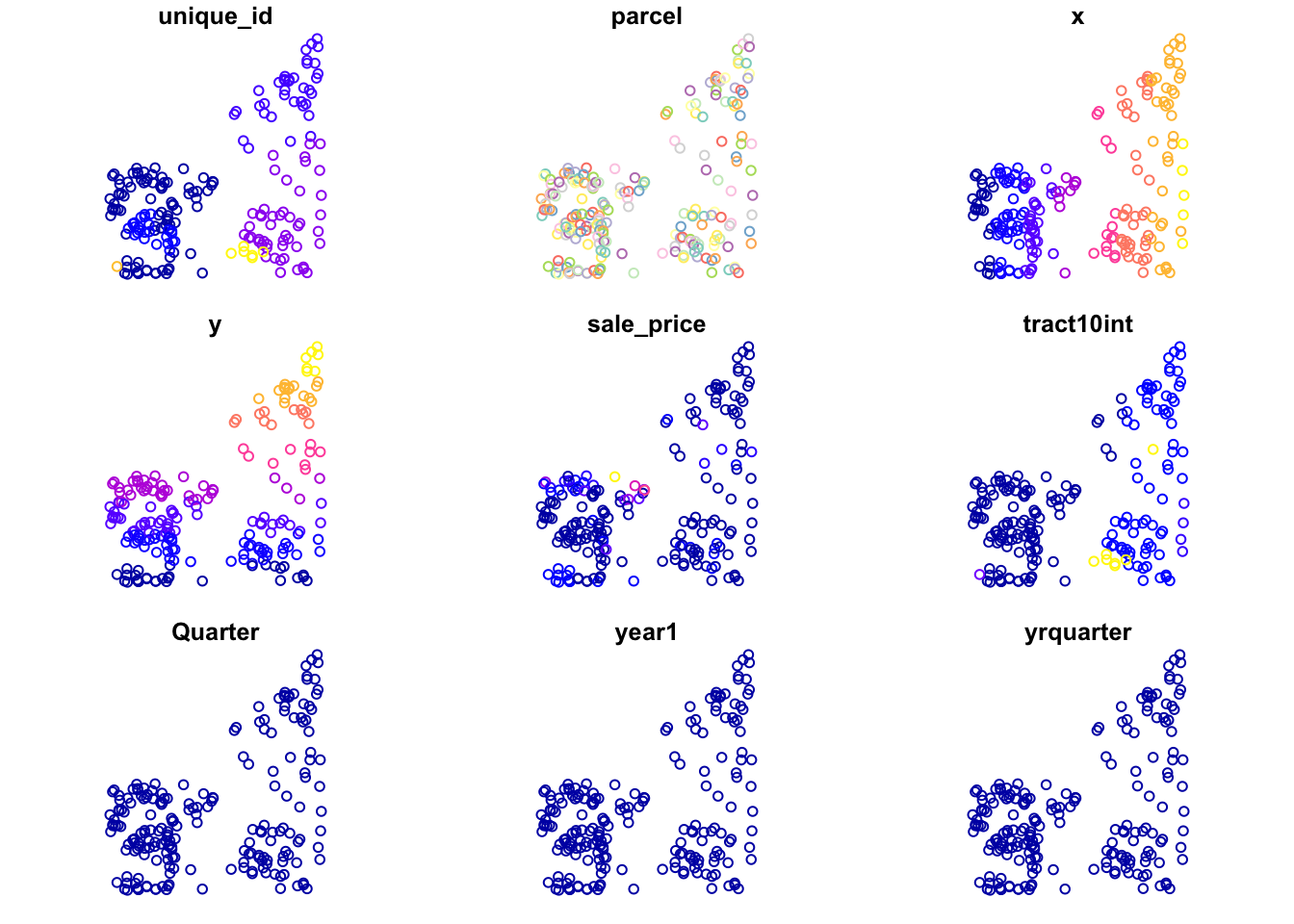
Visualizing point data
To get a cursory look at the point data with a basemap, we will use tmap. To get this done we first have to switch from mode plot to mode view with the function tmap_mode. From there we use tm_shape and tm_dots to display our points on the basemap. The only argument we need to pass is the shapefile into the tm_shape function.
tmap_mode("view")## tmap mode set to interactive viewingtm_shape(clev.points) +
tm_dots()Now we switch back to plot mode for the rest of the notebook with tmap_mode("plot").
tmap_mode("plot")## tmap mode set to plottingDistance-Band Weights
Concepts
Distance Metric
The core input into the determination of a neighbor relation for distance-based spatial weights is a formal measure of distance, or a distance metric. The most familiar special case is the Euclidean or straight line distance, \(d_{ij}\), as the crow flies: \[ d_{ij} = \sqrt{(x_i-x_j)^2 + (y_i - y_j)^2}\]
for two points i and j with respective coordinates \((x_i,y_i)\) and \((x_j,y_j)\).
Great Circle distance
Euclidean inter-point distances are only meaningful when the coordinates are recorded on a plane, i.e., for projected points.
In practice, one often works with unprojected points, expressed as degrees of latitude and longitude, in which case using a straight line distance measure is inappropriate, since it ignores the curvature of the earth. This is especially the case for longer distances, such as from the East Coast to the West Coast in the U.S.
The proper distance measure in this case is the so-called arc distance or great circle distance. This takes the latitude and longitude in decimal degrees as input into a conversion formula.3 Decimal degrees are obtained from the degree-minute-second value as degrees + minutes/60 + seconds/3600.
The latitude and longitude in decimal degrees are converted into radians as:
\[Lat_r = (Lat_d - 90) * \pi/180\] \[Lon_r = Lon_d * \pi/180\]
where the subscripts d and r refer respectively to decimal degrees and radians, and π=3.14159… With \(\Delta Lon = Lon_r(j)- Lon_r(i)\), the expression for the arc distance is:
\[d_{ij} = R * arccos[cos(\Delta Lon) * sin(Lat_{r(i)}) * sin(Lat_{r(j)}) + cos(Lat_{r(i)}) * cos(Lat_{r(j)})]\] or equivalently:
\[d_{ij} = R * arccos[cos(\Delta Lon) * cos(Lat_{r(i)}) * cos(Lat_{r(j)}) + sin(Lat_{r(i)}) * sin(Lat_{r(j)})]\]
where R is the radius of the earth. In GeoDa, the arc distance is obtained in miles with R = 3959, and in kilometers with R = 6371.
These calculated distance values are only approximate, since the radius of the earth is taken at the equator. A more precise measure would take into account the actual latitude at which the distance is measured. In addition, the earth’s shape is much more complex than a sphere, but the approximation serves our purposes.
Distance-band weights
The most straightforward spatial weights matrix constructed from a distance measure is obtained when i and j are considered neighbors whenever j falls within a critical distance band from i. More precisely, \(w_{ij}=1\) when $d_{ij} $ , and \(w_{ij}=0\) otherwise, where \(\delta\) is a preset critical distance cutoff.
In order to avoid isolates (islands) that would result from too stringent a critical distance, the distance must be chosen such that each location has at least one neighbor. Such a distance conforms to a max-min criterion, i.e., it is the largest of the nearest neighbor distances.
In practice, the max-min criterion often leads to too many neighbors for locations that are somewhat clustered, since the critical distance is determined by the points that are furthest apart. This problem frequently occurs when the density of the points is uneven across the data set, such as when some of the points are clustered and others more spread out. We revisit this problem in the illustrations below.
Creating distance-band weights
In order to start the distance based neighbors, we first need to compute a threshold value(The minimum distance that gives each point at least one neighbor). We can find this using k-nearest neighbors, which will be covered in more depth later in the notebook. We find the list of k-nearest neighbors for k = 1 then find the max distance between two neighbors in this list, which we then use as the upper distance parameter in the dnearneigh.
Computing Critical Threshold
Before we move forward, we need to x and y coordinates in a matrix. This is easily done by using cbind on the x and y coordinate columns of clev.points. cbind puts together vectors as columns in a matrix, so it is perfect for this task.
coords <- cbind(clev.points$x,clev.points$y)To find the critical threshold, we first find the k-nearest neighbors for k = 1. This will give us a list, where each point has exactly one neighbor. To do this, we use the ’knearneigh` function from spdep library. This will give a class of knn, which is similar to class nb, but will need to be converted anyways.
knn1 <- knearneigh(coords)Here we take a comprehensive look at our resulting knn object with the str command.
str(knn1)## List of 5
## $ nn : int [1:205, 1] 2 1 5 5 4 5 8 7 10 9 ...
## $ np : int 205
## $ k : num 1
## $ dimension: int 2
## $ x : num [1:205, 1:2] 2177340 2177090 2182100 2181090 2181090 ...
## - attr(*, "class")= chr "knn"
## - attr(*, "call")= language knearneigh(x = coords)Now we convert to nb. This simple, as there is a built in function for it in the spdep library: knn2nb.
k1 <- knn2nb(knn1)Computing the critical threshold will require a few functions, now that we have a neighbors list. First step is to get the distances between each point and it’s closest neighbor. This can be done with the nbdists. With these distances, we just need to find the maximum. For this we use the max command. However, we cannot do this with lists, so we must first get a data type that works for the max command, in our case, we use unlist
critical.threshold <- max(unlist(nbdists(k1,coords)))
critical.threshold
## [1] 3598.055Computing distance-band weights
With our critical threshold, we have a baseline value to work with for our distance-band neighbors. To make this neighbor’s list we use dnearneigh from the spdep package. The parameters necessary are the coordinates, the lower distance bound, and the upper distance bound. We enter these in the the above order. Another important parameter is the longlat. This is used for point data in longitude and latitude form. It is necessary to use this to get great circle distance instead of euclidean for accuracy purposes.
nb.dist.band <- dnearneigh(coords, 0, critical.threshold)Weights characteristics
We can examine the characteristics of these weights through a connectivity graph, connectivity histogram, and summary statistics.
Weights summary
We can use the base R summary command to get a comprehensive look at our distance-band weights object. This will give us a lot of useful information, that we cannot get with the str command.
summary(nb.dist.band)## Neighbour list object:
## Number of regions: 205
## Number of nonzero links: 2592
## Percentage nonzero weights: 6.167757
## Average number of links: 12.6439
## Link number distribution:
##
## 1 2 3 4 5 6 7 8 9 10 11 12 13 14 15 16 17 18 19 20 21 22 23 24 25
## 6 6 9 5 5 10 8 10 13 12 11 6 17 8 9 11 13 6 10 7 2 4 6 2 1
## 26 27 28 29 30 32
## 1 1 2 1 1 2
## 6 least connected regions:
## 59 114 115 116 117 198 with 1 link
## 2 most connected regions:
## 82 88 with 32 linksConnectivity histogram
Our method for making connectivity histograms will be the same as for contiguity based weights. We first need to get the cardinality for each observation(the number of neighbors for each observation). This is done by the card function from the spdep library. Our result from this function will be a vector of the number of neighbors for each location.
dist.band.card <- card(nb.dist.band)
dist.band.card
## [1] 9 9 15 15 15 17 15 15 19 18 20 20 20 19 14 17 17 19 13 3 9 10 7
## [24] 6 6 12 10 10 10 13 16 17 12 16 14 17 9 11 13 11 16 14 17 17 18 13
## [47] 13 17 18 16 16 24 27 22 17 8 7 6 1 11 11 11 11 11 13 13 13 13 13
## [70] 16 16 14 14 13 13 10 10 9 10 23 25 32 28 28 26 23 23 32 23 23 21 24
## [93] 18 18 17 21 15 20 20 22 19 22 22 19 16 18 20 19 19 23 19 29 30 1 1
## [116] 1 1 3 5 3 3 4 9 9 9 9 11 10 11 13 11 8 9 12 16 10 9 7
## [139] 6 6 3 6 8 8 7 7 7 4 6 5 5 3 2 2 2 7 8 8 10 8 6
## [162] 3 2 2 3 2 6 7 8 10 14 14 12 17 16 16 20 19 19 13 17 13 15 12
## [185] 11 14 5 8 9 8 10 12 6 5 4 3 4 1 9 4 13 13 15 15 17Once, we have our cardinality, we can make a histogram to see the distribution of the number of neighbors. we will do this with ggplot2, though base R also has a built in histogram function. To make our histogram, we start with the ggplot function, then add a histogram layer. We add the additional layer with the + operator. Next, we use geom_histogram to add our histogram. The only parameter we need is an aes. We use the aes function and enter our cardinality(dist.band.card) as the variable for the x-axis. Beyond this, we change the x-axis label to be more informative with the xlab function.
ggplot() +
  geom_histogram(aes(x=dist.band.card)) +
  xlab("Number of Neighbors")
## `stat_bin()` using `bins = 30`. Pick better value with `binwidth`.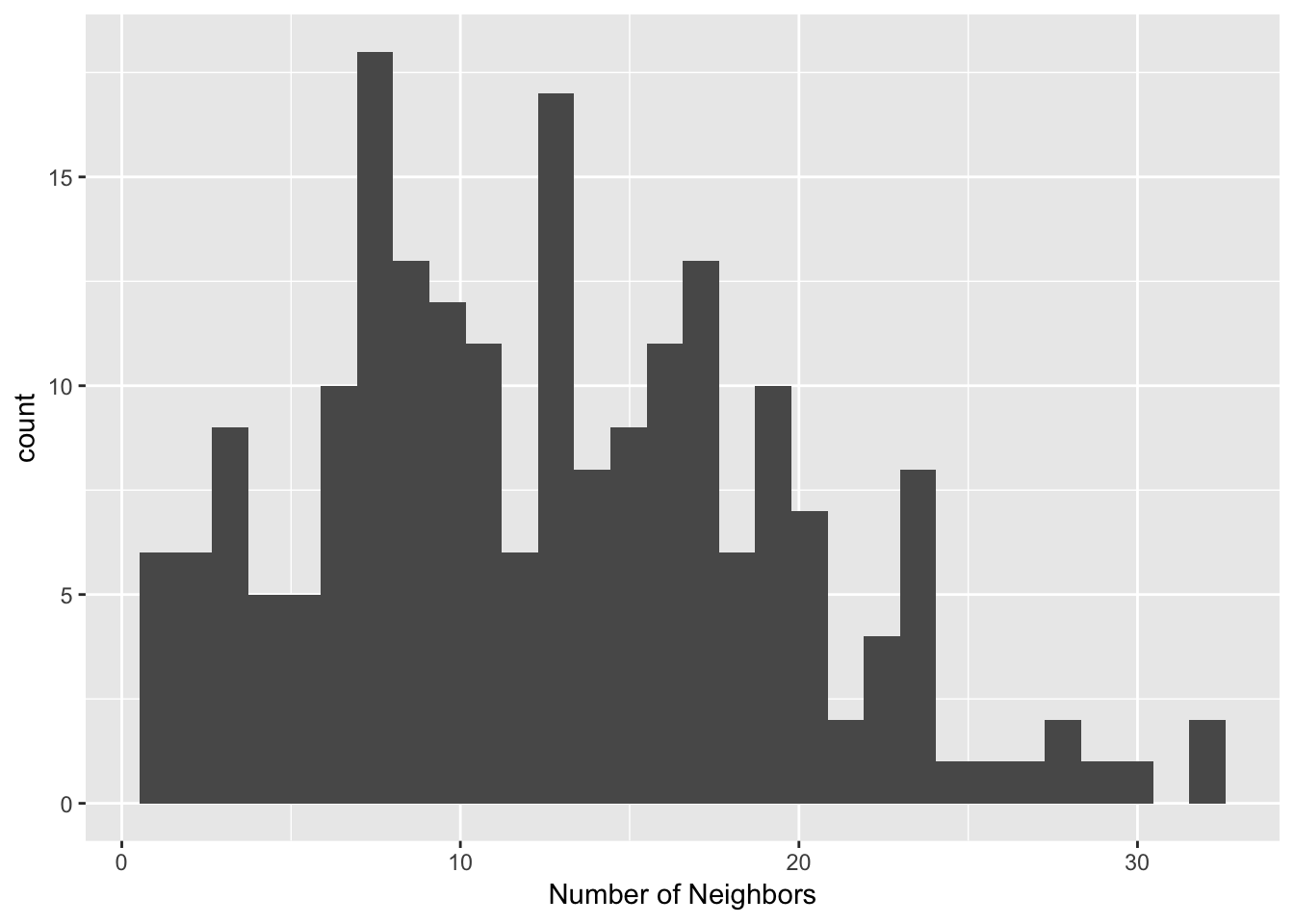
Connectivity graph
For our connectivity graph, we follow the same steps as for the contiguity weights. We use the plot command and use our neighbors list and coordinates as inputs. We use additional parameters to make the graph easier to look at. We shorten the line width with lwd =.2 and make the points smaller with cex = .5. The default points are much to big, and it is hard to get sense of the graphs structure.
plot(nb.dist.band, coords, lwd=.2, col="blue", cex = .5)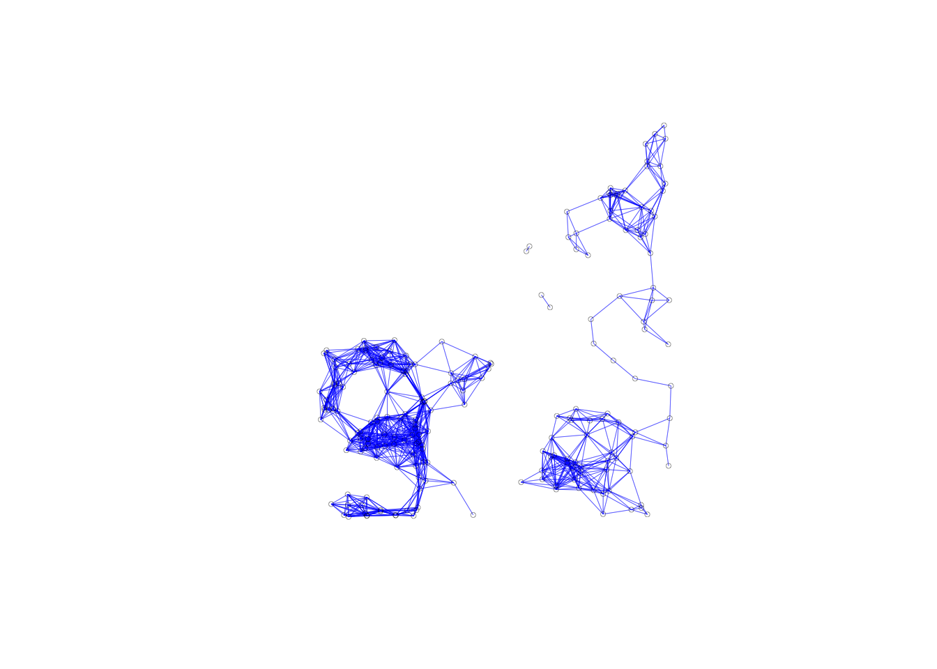
We can see that we have no isolates from our graph, as we expect from using a critical threshold approach. Our graphs structure consists of two subgraphs and two pairs of points.
Isolates
So far, we have used the default cut-off value for the distance band. However, the function is flexible enough that we can type in any value for the cut-off, or use the movable button to drag to any value larger than the minimum. Sometimes, theoretical or policy considerations suggest a specific value for the cut-off that may be smaller than the max-min distance.
From our example we know the critical threshold is 3598, so we can pick a value lower to get some isolates in our distance-band weights. We will use 1500 ft, same as the corresponding GeoDa workbook example.
The only change we need to make to do this, is make the upper distance bound 1500, instead of critical.threshold.
dist.band.iso <- dnearneigh(coords, 0, 1500)Isolates in the connectivity histogram
We can get a measure of the number of isolates by looking at the left most bar of a connectivity histogram. To make this, we follow the same procedure as the earlier connectivity histograms. We first get the cardinality, then use ggplot2 to make the histogram.
iso.card <- card(dist.band.iso)ggplot() +
geom_histogram(aes(x=iso.card)) +
xlab("Number of Neighbors")## `stat_bin()` using `bins = 30`. Pick better value with `binwidth`.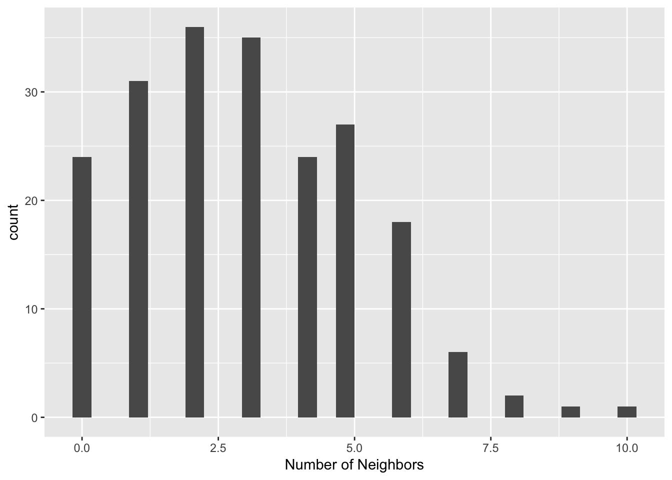 Our resulting histogram has 24 isolates, and is much more compact than the original one with the critical threshold as the upper distance bound in our distance-band weights.
Isolates in the connectivity graph
The most dramatic visualization of the isolates is given by the connectivity graph. The 24 points without an edge to another point are easily identified
plot(dist.band.iso, coords, lwd=.2, col="blue", cex = .5)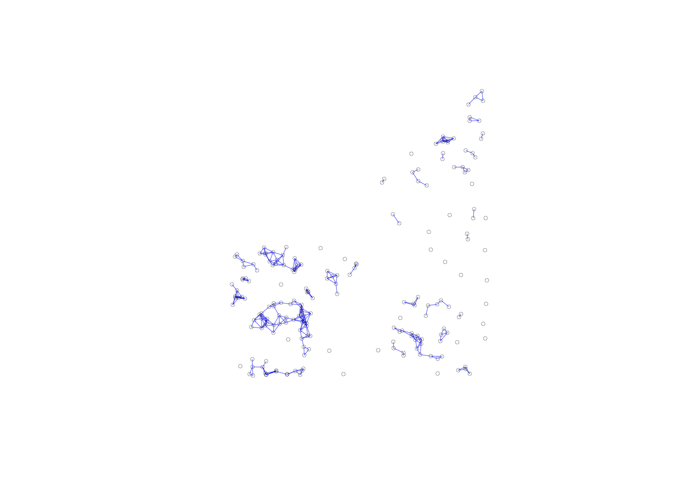
How to deal with isolates
Since the isolated observations are not included in the spatial weights (in effect, the corresponding row in the spatial weights matrix consists of zeros), they are not accounted for in any spatial analysis, such as tests for spatial autocorrelation, or spatial regression. For all practical purposes, they should be removed from such analysis. However, they are fine to be included in a traditional non-spatial data analysis.
Ignoring isolates may cause problems in the calculation of spatially lagged variables, or measures of local spatial autocorrelation. By construction, the spatially lagged variable will be zero, which may suggest spurious correlations.
Alternatives where isolates are avoided by design are the K-nearest neighbor weights and contiguity weights constructed from the Thiessen polygons for the points. They are discussed next.
K-Nearest Neighbor Weights
Concept
As mentioned, an alternative type of distance-based spatial weights that avoids the problem of isolates are k-nearest neighbor weights. In contrast to the distance band, this is not a symmetric relation. The fact that B is the nearest neighbor to A does not imply that A is the nearest neighbor to B. There may be another point C that is actually closer to B than A. This asymmetry can cause problems in analysis that depend on the intrinsic symmetry of the weights (e.g., some algorithms to estimate spatial regression models). One solution is to replace the original weights matrix W by (W+W′)/2, which is symmetric by construction. GeoDa currently does not implement this approach.
A potential issue with k-nearest neighbor weights is the occurrence of ties, i.e., when more than one location j has the same distance from i. A number of solutions exist to break the tie, from randomly selecting one of the k-th order neighbors, to including all of them. In GeoDa, random selection is implemented.
Creating KNN Weights
To create our KNN weights, we need two functions from the spdep library: knearneigh and knn2nb. We first use knearneigh to get a class of knn, as we did earlier to find the critical threshold. This time we assign k = a value of 6. This means each observation will get a list of the 6 closest points. We then use knn2nb to convert from class knn to class nb.
k6 <- knn2nb(knearneigh(coords, k = 6))Properties of KNN weights
One drawback of the k-nearest neighbor approach is that it ignores the distances involved. The first k neighbors are selected, irrespective of how near or how far they may be. This suggests a notion of distance decay that is not absolute, but relative, in the sense of intervening opportunities (e.g., you consider the two closest grocery stores, irrespective of how far they may be).
Again, we can also use the connectivity histogram and the connectivity map to inspect the neighbor characteristics of the observations. However, in this case, the histogram doesn’t make much sense, since all observations have the same number of neighbors, as shown by our histogram.
k6.card <- card(k6)
ggplot() +
  geom_histogram(aes(x=k6.card), binwidth = .01) +
  xlab("Number of Neighbors")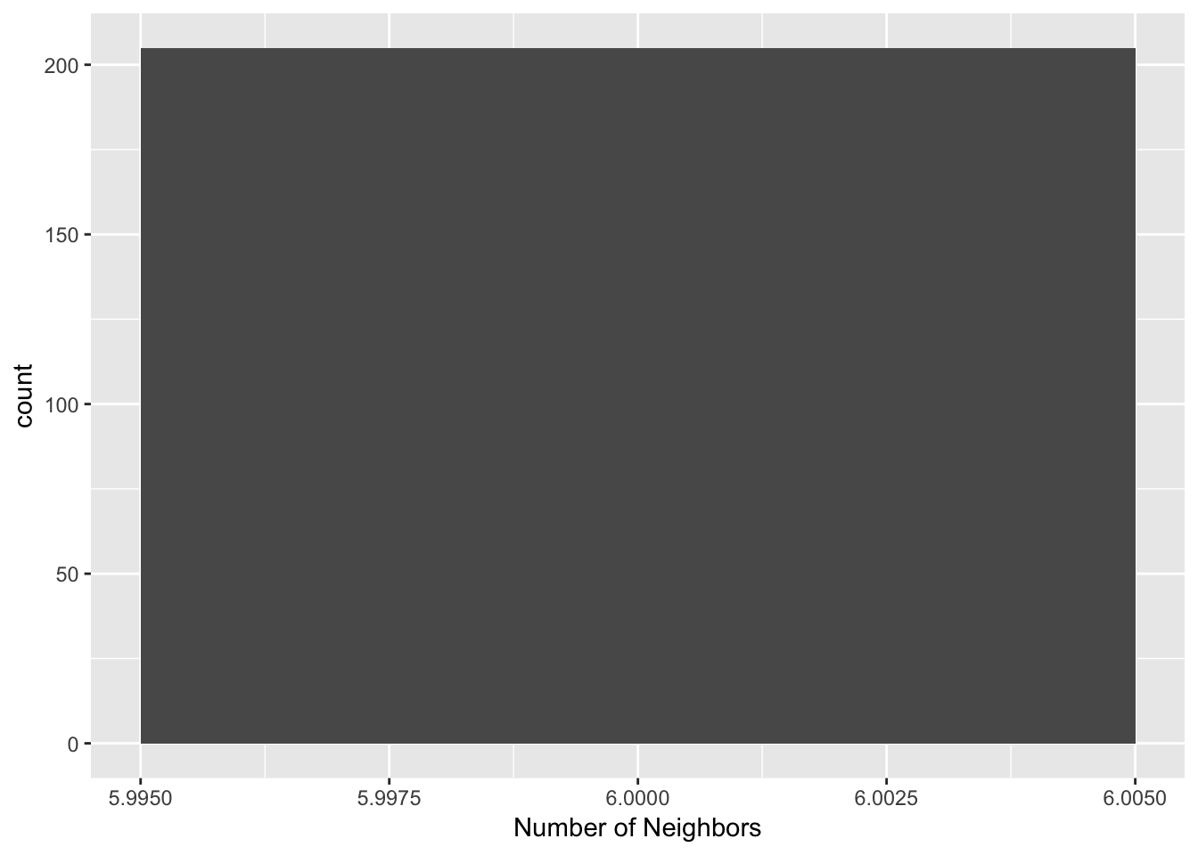
In contrast, the connectivity graph, clearly demonstrates how each point is connected to six other points. In our example, this yields a fully connected graph instead of the collection of sub-graphs for the distance band.
plot(k6, coords, lwd=.2, col="blue", cex = .5)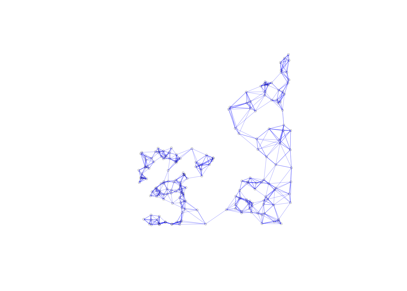
Generalizing the Concept of Contiguity
In GeoDa, the concept of contiguity can be generalized to point layers by converting the latter to a tessellation, specifically Thiessen polygons. Queen or rook contiguity weights can then be created for the polygons, in the usual way.
Similarly, the concepts of distance-band weights and k-nearest neighbor weights can be generalized to polygon layers. The layers are represented by their central points and the standard distance computations are applied.
We can apply these concepts through R computations, in a similar manner as GeoDa, but it will take more steps.
Contiguity-based weights for points
Thiessen polygons
An alternative solution to deal with the problem of the uneven distribution of neighbor cardinality for distance-band weights is to compute a measure of contiguity. This is accomplished by turning the points into Thiessen polygons. These are also referred to as Voronoi diagrams or Delaunay triangulations.
In general terms, a Thiessen polygon is a tessellation (a way to divide an area into regular subareas) that encloses all locations that are closer to the central point than to any other point. In economic geography, this is a (simplistic) notion of a market area, in the sense that all consumers in the polygon would patronize the seller located at the central point. The polygons are constructed by combining lines perpendicular at the midpoint of a line that connects a point to its nearest neighbors. From this, the most compact polygon is created.
Creating Thiessen polygons from a point layer
To create the Thiessen polygons, we will use the deldir package, then will convert them to a data form that we can use for the contiguity weights. We won’t go into too much detail about the deldir package, other than how to create the polygons and convert them to sp, then sf. For more information on the deldir, visit deldir documentation.
To create our Thiessen polygons from the deldir function, we just need a vector with x coordinates and a vector with y coordinates. From there we can use the plot command to visualize these because here is a built in method for deldir Thiessen polygons. To get a good visual of our polygons, we need a few extra parameters. These are: wlines, wpoints, and lty. wlines = "tess" gets us the basic polygons. wpoints = "none" keeps points off the map. lty = 1 specifies a solid line type.
vtess <- deldir(clev.points$x, clev.points$y)##
## PLEASE NOTE: The components "delsgs" and "summary" of the
## object returned by deldir() are now DATA FRAMES rather than
## matrices (as they were prior to release 0.0-18).
## See help("deldir").
##
## PLEASE NOTE: The process that deldir() uses for determining
## duplicated points has changed from that used in version
## 0.0-9 of this package (and previously). See help("deldir").plot(vtess, wlines="tess", wpoints="none",
lty=1)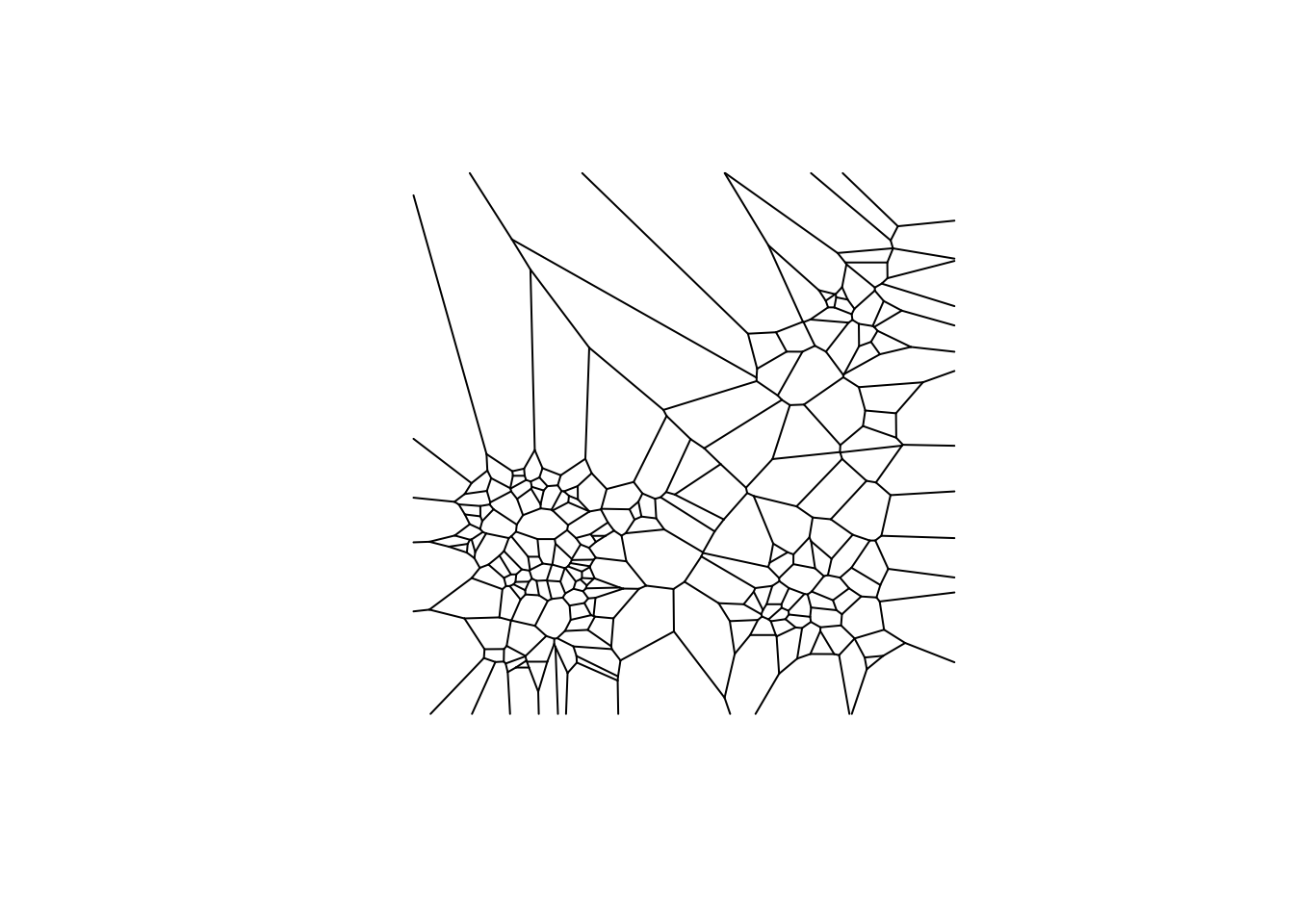
The function below converts class deldir to sp. We will not go in depth on the structure and set up of this function because it goes to heavy into sp, and these notebooks are primarily focused on sf.
voronoipolygons = function(thiess) {
w = tile.list(thiess)
polys = vector(mode='list', length=length(w))
for (i in seq(along=polys)) {
    pcrds = cbind(w[[i]]$x, w[[i]]$y)
    pcrds = rbind(pcrds, pcrds[1,])
    polys[[i]] = Polygons(list(Polygon(pcrds)), ID=as.character(i))
}
SP = SpatialPolygons(polys)
 voronoi = SpatialPolygonsDataFrame(SP, data=data.frame(dummy = seq(length(SP)), row.names=sapply(slot(SP, 'polygons'),
    function(x) slot(x, 'ID'))))
}
The result of our function is a SpatialPolygonsDataFrame, which is a class from the sp package. We will convert again to get to the sf class, since sf is more efficient and accurate. We check our function by plotting the result and get something similar to what we plotted earlier, just now it is a different data structure.
v <- voronoipolygons(vtess)## Warning in seq.default(along = polys): partial argument match of 'along' to
## 'along.with'plot(v)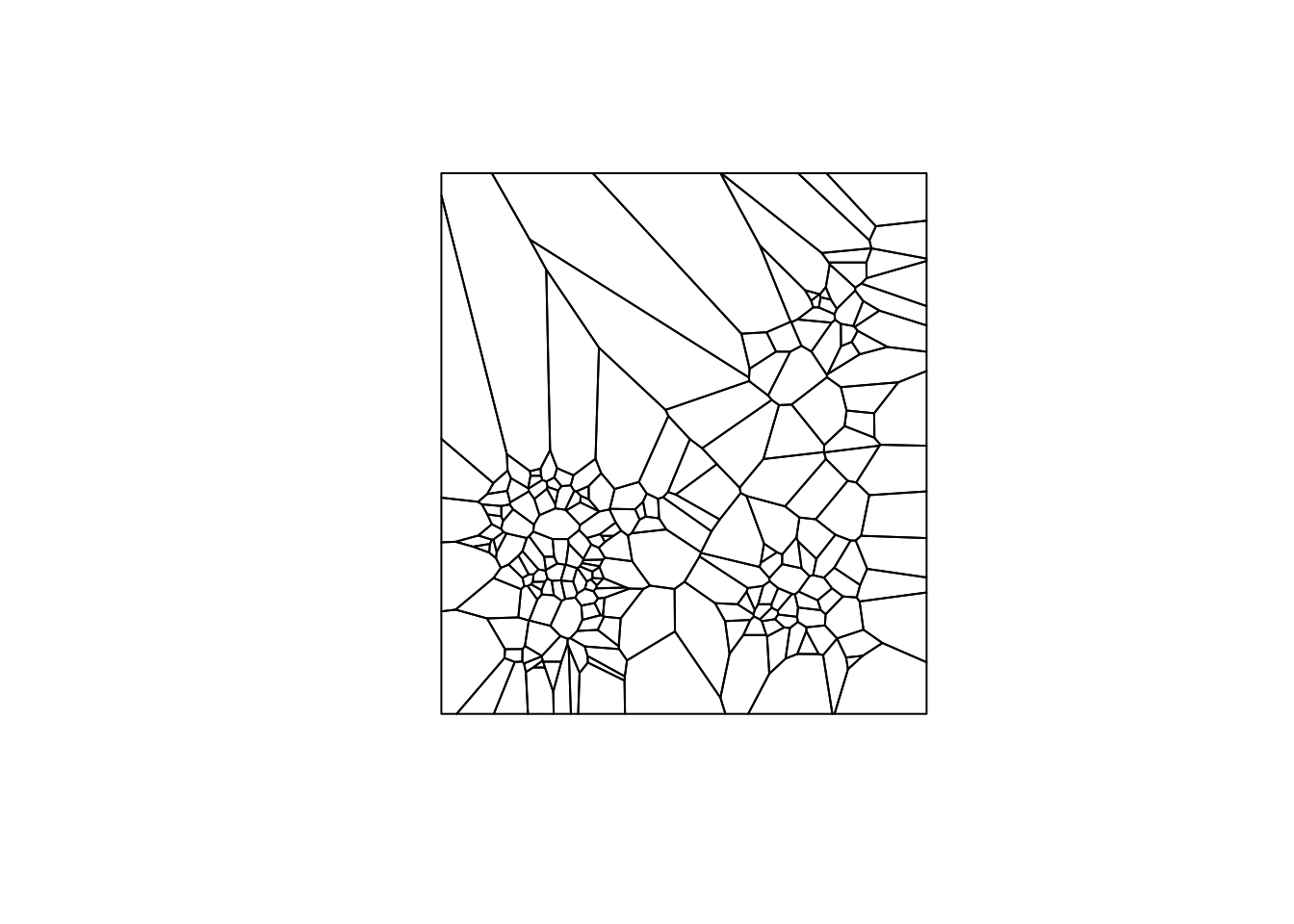
Using the sf function st_as_sf, we can convert to sf from our SpatialPolygonsDataFrame. Again, we use the plot command to check our result.
vtess.sf <- st_as_sf(v)
plot(vtess.sf$geometry)
Contiguity weights for Thiessen polygons
To make our queen contiguity weights, we make a function using st_relate and specifying a DE9-IM pattern. For queen contiguity, our pattern is "F***T****". We don’t really need to go into why the pattern is what it is for our purposes, but DE9-IM and st_relate documentation can help explain this to a degree.
st_queen <- function(a, b = a) st_relate(a, b, pattern = "F***T****")Here we use our function to get a neighbor list of class sgbp, which stands for sparse geometry binary predicate. In order to use the spdep library, we will have to convert to class nb, as done in the contiguity weights notebook.
queen.sgbp <- st_queen(vtess.sf)Now we will we start our conversion from class sgbp to nb. To do this, we need to change the class explicitly and take the precaution to represent observations with no neighbors with the integer 0. Our data set doesn’t have any observations without neighbors, but in ones with these, it will mess everything up, if not dealt with.
We start with the function operator. The input for our function will be an object of class sgbp, denoted by x. We store the attributes in attrs, as we will need to reapply them later. Now we deal we observation with no neighbors. We will use lapply, which applies a function to each element of a list or vector. As for the input function, we make one that checks the length of an element of our list for 0(meaning no neighbors) and returns 0 if the element is empty and the element otherwise. This can be a bit confusing, for more information on lapply, check out lapply documentation
From here we will have dealt with observations with no neighbors, but will need to reapply our attributes to the resulting structure from the lapply function. This is done by calling the attributes function and assigning the stored attributes. The final step is to explicitly change the class to nb by using the class function and assigning "nb". We then return our object x.
as.nb.sgbp <- function(x, ...) {
  attrs <- attributes(x)
  x <- lapply(x, function(i) { if(length(i) == 0L) 0L else i } )
  attributes(x) <- attrs
  class(x) <- "nb"
  x
}
With our conversion function, we can covert to class nb.
queen.nb <- as.nb.sgbp(queen.sgbp)We can take a look at the distribution of the number of neighbors in our queen contiguity for the Thiessen polygons with a connectivity histogram. The steps are the same as earlier for all the other connectivity histograms
queen.nb.card <- card(queen.nb)
ggplot() +
  geom_histogram(aes(x=queen.nb.card)) +
  xlab("Number of Neighbors")
## `stat_bin()` using `bins = 30`. Pick better value with `binwidth`.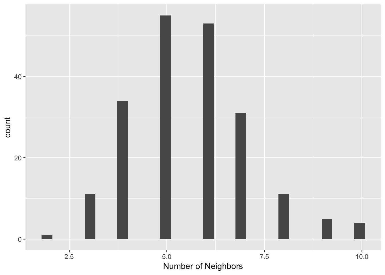
summary(queen.nb)## Neighbour list object:
## Number of regions: 205
## Number of nonzero links: 1154
## Percentage nonzero weights: 2.745985
## Average number of links: 5.629268
## Link number distribution:
##
## 2 3 4 5 6 7 8 9 10
## 1 11 34 55 53 31 11 5 4
## 1 least connected region:
## 141 with 2 links
## 4 most connected regions:
## 36 57 87 96 with 10 linksThe histogram and summary statistics represents a much more symmetric and compact distribution of the neighbor cardinalities, very similar to the typical shape of the histogram for first order contiguity between polygons. The median number of neighbors is 6 and the average 5.6, with a limited spread around these values. In many instances where the point distribution is highly uneven, this approach provides a useful compromise between the distance-band and the k-nearest neighbors.
This will be further illustrated through a connectivity graph with a far more balanced structure.
plot(queen.nb,coords, lwd=.2, col="blue", cex = .5)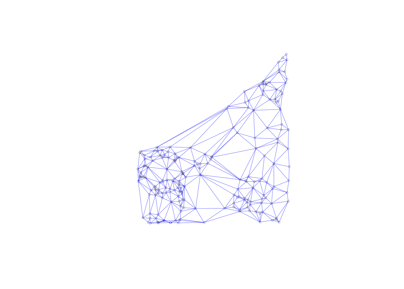
Distance-based weights for polygons
As we can do contiguity-based weights for point data, we use distance-based weights for polygons. To illustrate this, we will use U.S homicide data from a previous notebook(the contiguity-based weights notebook).
To implement this we start by computing shape center coordinates for the polygons. Once we get the coordinates, we will follow the procedure for making distance-band weights. There will be one key difference, as we will be working with nonprojected data. We will have to use great circle distance instead of euclidean. The formulas for these were went over earlier, in the notebook, but working with this difference requires only a few changes in the steps to make distance-band neighbors.
Getting the data
To get the data, we will use the geodaData package again. Additionally, the data for this notebook can be found at US Homicides. If the data is downloaded directly, then you must put it in your working directory and load it with st_read.
us.bound <- geodaData::ncovrComputing the centroids
Getting our coordinate data is a little more complicate than just using st_centroid on our shapefile. We need to do this to get coordinates in a supported format for the neighbor functions in the *spdep** package. We are going to get vectors for latitude and longitude, then will bind the columns for later use.
To get our centroid coordinates, we will map the function st_centroid over the geometry column of us.bound. The mapping function applies a given function to each element of a vector and returns a vector of the same length. Our input vector will be the geometry column of us.bound. Our function will be st_centroid. We will use the map_dbl variation of map from the purrr package. For more documentation, check out map documentation
latitude <- map_dbl(us.bound$geometry, ~st_centroid(.x)[[1]])We do the same for latitude, using [[2]] to get the latitude values.
longitude <- map_dbl(us.bound$geometry, ~st_centroid(.x)[[2]])Now we bind the coordinates together with cbind, so we can enter them as parameters in the neighbors functions.
center.coords <- cbind(latitude,longitude)Computing the critical threshold
To get the critical threshold, we follow the same steps as earlier, with one difference. This time we will set longlat = TRUE in three of the functions. This is important because our data is not projected and to get accurate results we must work with great circle distance.
Again we begin with finding the first nearest neighbors and convert from class knn to class nb, and set longlat = TRUE.
k.poly <- knn2nb(knearneigh(center.coords, longlat = TRUE))After we have computed the first nearest neighbors, we find the maximum distance in this neighbors list, so our distance-band weights will not have isolates. For our distance function: nbdists we also need to set longlat = TRUE. This is needed here, as we are calculating the distances between each set of points.
critical.threshold.poly <- max(unlist(nbdists(k.poly,center.coords, longlat = TRUE)))Computing distance-band neighbors
We now have all the components necessary to do the distance-band weight for our polygon data. Again we use dnearneigh to get our distance-band weights. We input the centroid coordinates, a distance lower bound(0), a distance upper bound(the critical threshold), and set longlat = TRUE.
nb.dist.band.poly <- dnearneigh(center.coords, 0, critical.threshold.poly, longlat = TRUE)Once we have calculated the distance-band weights, we can assess the distribution of the number of neighbors through a connectivity histogram, following the same procedure used through the notebook.
poly.nb.card <- card(nb.dist.band.poly)
ggplot() +
  geom_histogram(aes(x=poly.nb.card)) +
  xlab("Number of Neighbors")
## `stat_bin()` using `bins = 30`. Pick better value with `binwidth`.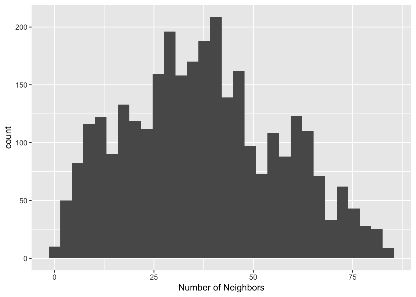
University of Chicago, Center for Spatial Data Science – anselin@uchicago.edu,morrisonge@uchicago.edu↩
Use
setwd(directorypath)to specify the working directory.↩Use
install.packages(packagename).↩