Columbus Crime 1980

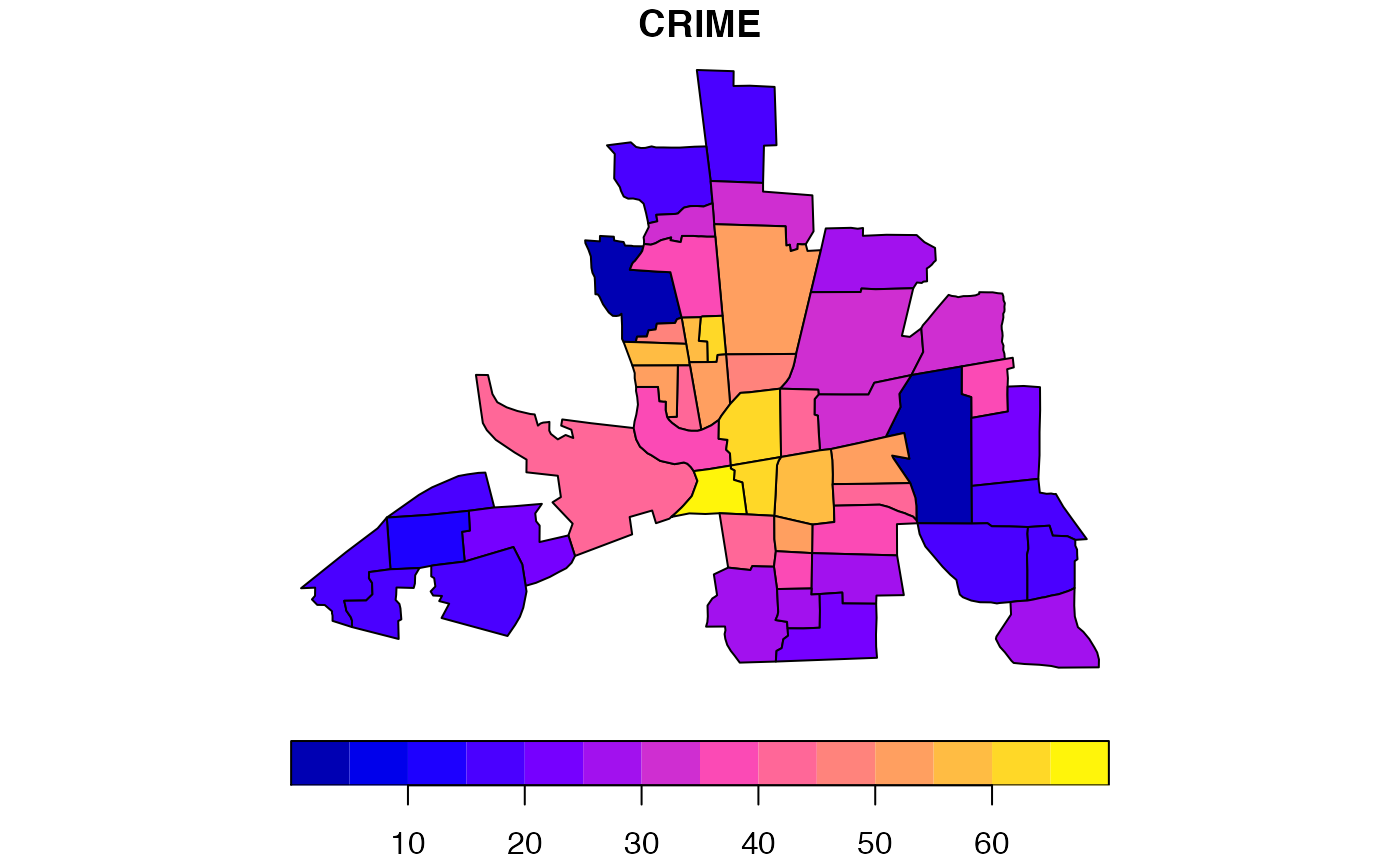
Crime, housing and income data for 49 neighborhoods in Columbus, OH, 1980. Textbook example.

columbus

Format

An sf data frame with 49 rows, 20 variables, and a geometry column:

AREA

neighborhood area (computed by ArcView)

PERIMETER

neighborhood perimeter (computed by ArcView)

COLUMBUS

internal polygon ID (generated by ArcView)

COLUMBUS_I

internal polygon ID (geneated by ArcView)

POLYID

neighborhood ID, used in GeoDa User’s Guide and tutorials

NEIG

neighborhood ID, used in Spatial Econometrics examples

HOVAL

housing value (in $1,000)

INC

household income (in $1,000)

CRIME

residential burglaries and vehicle thefts per 1000 households

OPEN

open space (area)

PLUMB

percent housing units without plumbing

DISCBD

distance to CBD

X

centroid x coordinate (in arbitrary digitizing units)

Y

centroid y coordinate (in arbitrary digitizing units)

NSA

north-south indicator variable (North = 1)

NSB

other north-south indicator variable (North = 1)

EW

east-west indicator variable (East = 1)

CP

core-periphery indicator variable (Core = 1)

THOUS

constant (= 1000)

NEIGNO

another neighborhood ID variable (NEIG + 1000)

Source

Anselin, Luc (1988). Spatial Econometrics. Boston, Kluwer Academic, Table 12.1, p. 189.

Details

Sf object, unprojected. EPSG 4326: WGS84.

Examples

if (requireNamespace("sf", quietly = TRUE)) {
  library(sf)
  data(columbus)

  plot(columbus["CRIME"])
}